R Programming Language

r fundamentals, packages, programming

2026-01-27

Welcome to R

R Programming Language

  • Built to efficiently store and manipulate data
  • Open-source, free, and flexible alternative to other statistical analysis software
  • Large, active community of users and contributors
  • Packages shared and stored on the open index CRAN (Comprehensive R Archive Network)

R: OOP

  • R is an object-oriented programming language (OOP)
    • Objects: contain a value and have an identifier
    • Classes: templates for objects and their contained data type
    • Structures: classes containing multiple objects
  • R manipulates data (objects)
    • Environments: collections of manipulable objects
    • Functions: procedures for creating or changing code
    • Arguments: inputs to functions that specify procedure

R Scripts

  • R scripts include:
    • Series of functions (code) to carry out in order
    • Plain text comments (non-code) that are ignored by R
  • R code is written in:
    • R script files (.R)
    • “Code chunks” within other file types (e.g., .Rmd & .qmd notebooks)
  • Sourcing scripts allows code in one file to “talk to” code in other files

R Syntax

Comments

  • Comments are plain text notes within code that are ignored by R
  • Created using the # symbol
    • Everything that follows on that line will be ignored
  • Used to:
    • Explain code functionality
    • Provide context or instructions
    • Temporarily disable code during testing/debugging
# This comment spans multiple lines. The `#` symbol must be used at the start 
# of each line. Alternatively, start the comment mid-line like below:

x <- 42  # The rest of this line is comment
# y <- x + 10  Treat this line as comment, not code

Variables

  • Variables store data values with unique identifiers
  • Created using the assignment operator <-
    • Example: class_name <- "D2M-R"
  • Variable names:
    • Are case-sensitive
      • e.g., Class_Name, class_name, and CLASS_NAME are different variables
    • MUST start with a letter or dot, not a number
      • e.g., student1, .temp_value are valid; 1student, _value are not
    • MUST contain (only) letters, numbers, dots, or underscores
      • e.g., total.score, data_frame_1 are valid; total-score, data frame are not
    • SHOULD be descriptive, meaningful, and pronounceable
      • e.g., student_age, is_enrolled, total_score
    • SHOULD follow consistent naming conventions

Main Data Types

Data you can work with in R takes one of 61 forms, most commonly:

Data type Description Example
Numeric Decimal numbers, including whole numbers 3.14, 42.0, -1.5
Integer Whole numbers (exclusively), represented with an L suffix 42L, -1L, 1000L
Logical Boolean values, either TRUE or FALSE TRUE, FALSE or T, F
Character Text strings, enclosed in quotes "hello", '123', "R is great!"

Data Types(+)

There are also a few “honorary” data types:

Data type Description Example
Factor Leveled categorical data, stored as integers with labels factor(c("low", "medium", "high"))
Date Dates, stored as a special class of object as.Date("2025-01-31")
POSIXct Date-time objects, which include both date and time as.POSIXct("1776-07-04 12:01:59")
empty Not a data type, but the absence of data NA

Data Structures

R organizes data into structures to for manipulation and analysis. The main data structures are:

Data structure Description Example
Scalar Single data value of any data type 42, "hello", TRUE
Vector One-dimensional array of elements of the same data type c(1, 2, 3, 4, 5)
List Ordered collection of elements that can be of different data types list(name = "Alice", age = 30, scores = c(90, 85, 88))
Matrix Two-dimensional array of elements of the same data type matrix(1:6, nrow = 2, ncol = 3)
Data Frame Two-dimensional, tabular data structure with columns of potentially different data types data.frame(name = c("Alice", "Bob"), age = c(30, 25))
Tibbles Alternative data frames with enhanced features tibble::tibble(name = c("Alice", "Bob"), age = c(30, 25))

Data Structures: Data Frames and Tibbles

  • Data frames are 2-dimensional, tabular data structures
    • dfs are the heart <3 of R
    • Special type of list
      • Each vector in the list is a column
      • All of equal length (e.g. same number of rows)
      • Can be different data types across vectors
      • Must be the same data type within a vector
  • Tibbles are alternatives to data frames
    • Special type of data frame
    • Used in the tidyverse ecosystem
    • Have some enhanced features (e.g., better printing, stricter subsetting rules)
    • Functionally equivalent to data frames (for our purposes)

Operators

Operators are symbols that perform operations on variables and values. The main types of operators in R are:

Operator type Description Example
Arithmetic Perform mathematical calculations +, -, *, /, ^
Relational Compare values and return logical results ==, !=, <, >, <=, >=
Logical Combine or negate logical values &, |, !
Assignment Assign values to variables <-, =, ->

Operators: Arithmetic

Arithmetic do math.

  • Input: numeric data
  • Output: numeric data
Operator Description Example Output
+ Addition 3 + 5 8
- Subtraction 10 - 4
* Multiplication 6 * 7 42
/ Division 20 / 4 5
^ Exponentiation (power) 2 ^ 3 8
%% Modulo (remainder of division) 10 %% 3 1

Operators: Relational

Relational or comparison operators compare objects and return a logical value (TRUE or FALSE). They are a special kind of logical operator.

  • Input: numeric, character, or logical data
  • Output: logical data
Operator Description Example Output
== Equal to 5 == 5 TRUE
!= Not equal to (“≠”) 5 != 3 TRUE
> Greater than 7 > 4 TRUE
< Less than 3 < 8 TRUE
>= Greater than or equal to 6 >= 6 TRUE
<= Less than or equal to 2 <= 5 TRUE

Warning: '==' != '='

The == operator checks for equality, while = is an (argument) assignment operator.

Operators: Logical

Logical operators combine and modify boolean values (TRUE or FALSE).

  • Input: logical data
  • Output: logical data
Operator Description Example Output
& “and”: both sides of the operators evaluate to TRUE TRUE & FALSE FALSE
| “or”: at least one side of the operator evaluates to TRUE TRUE | FALSE TRUE
! “not”: the opposite of something’s logical evaluation !TRUE FALSE

Operators: Other

Operator Description Example Output
<- Variable assignment operator x <- 5 Assigns the value 5 to the variable x
= Argument assignment operator round(3.14159, digits = 2) Assigns the value 2 to the digits argument of the round() function
: Create a sequence of integers 1:5 c(1, 2, 3, 4, 5)
[ ] Subset elements of a vector, list, or data frame by position or name list(first = 1, second = 2)[2] > $second > [1] 2
[[ ]] Extract a single element from a list by position or name list(first = 1, second = 2)[[2]] 2
$ Extract a single element from a list or data frame by name list(first = 1, second = 2)$second 2
|> or %>% Pipe operator to pass the output of one function as the input to another data |> filter(condition) Passes data as the first argument to filter()

Functions

  • Basic syntax: function_name(argument1, argument2, ...)
    • Example: paste("Hello", class_name)
  • Functions: pre-defined procedures that perform specific tasks
    • Take 0 or more arguments as inputs
    • Return 1 output
  • Arguments: inputs to functions that specify procedure
    • Can be required or optional
    • Assigned with = operator or by position following default order
      • round(3.14159) is the same as round(x = 3.14159)
      • round(2, 3.14159) is not the same as round(digits = 2, x = 3.14159).
  • View all possible arguments in a function’s documentation with ?functionname or ??functionname.

Function Definition

All functions have:

  1. Name
  2. Zero or more arguments (inputs)
  3. Procedure body (code)
  4. Return value (output)
# See the elements of a function by running the name of 
# the function without parentheses in the console

example.function
<srcref: file "" chars 2:21 to 9:1>

Defining Functions

Use the function() function to define your own functions:

function_name <- function(arguments) {
    # Informative comments
    the code for your function
    return(value)
}
helloworld <- function(name, punctuation = "!") {
    # Prints greeting with name and punctuation
    greeting <- paste0("Hello ", name, punctuation)
    return(greeting)
}
# Specify both arguments in order 
# No argument names
helloworld("D2M-R", "!?")
[1] "Hello D2M-R!?"
# Specify arguments out of order 
# Use argument names
helloworld(
    punctuation = "...", 
    name = "class"
)
[1] "Hello class..."
# Specify required argument only
# Use default for optional
helloworld("everyone")
[1] "Hello everyone!"

Notes on Function Definition: Names, Arguments

Names

  • Descriptive, pronounceable, consistently styled
  • Unique within your R environment

Arguments

  • Typically limited to specific data types (e.g., numeric, character)
    • Data constraints can be explicitly checked with code or implicitly based on function body requirements
  • Can have default values assigned, making them optional
  • Specify arguments without naming them by following documented order: function_name(value1, value2)
  • Specify arguments out of order by naming them: function_name(arg2 = value2, arg1 = value1)

Notes on Function Definition: Body, Return

Procedure Body

  • Can include multiple lines of code and comments
  • Scoped environment: variables created inside are not accessible outside

Return Value

  • If specified with return(), that value is printed to console
    • return(arg1 + arg2) returns sum of arg1 and arg2
  • If no return() is used, the last evaluated expression is returned by default
    • arg1 + arg2 returns sum of arg1 and arg2
  • Functions have to evaluate without object assignment to return a value to the console
    • result <- arg1 + arg2 does not return anything

Reference: Useful Base R Functions (1)

Function Description Example Output
c() Combine values into a vector c(1, 2, 3) c(1, 2, 3)
paste() Concatenate strings together paste("Hello", "world!")
data.frame() Create a data frame from vectors data.frame(x = 1:3, y = c("a", "b", "c")) A data frame with 3 rows and 2 columns named x and y
class() Check the data type of an object class(3.14) "numeric"
str() Display the structure of an object str(mtcars) A summary of the mtcars data frame
length() Get the length of a vector length(c(1, 2, 3, 4, 5)) 5
head() View the first few rows of a data frame or vector head(mtcars) The first 6 (default) rows of the mtcars data frame
summary() Get a summary of a data frame or vector summary(mtcars) Summary statistics for each column in the mtcars data frame

Reference: Useful Base R Functions (2)

number_list <- c(11, 37, 42, 101, 202, 1000, 2025, -3)
Function Description Example Output
round() Round a numeric value to a specified number of decimal places round(67.1988, 2) 67.2
sum() Calculate the sum of a numeric vector sum(number_list) 3415
min() Find the minimum value in a numeric vector min(number_list) -3
max() Find the maximum value in a numeric vector max(number_list) 2025

Reference: Useful Base R Functions (3)

number_list <- c(11, 37, 42, 101, 202, 1000, 2025, -3)
Function Description Example Output
mean() Calculate the mean of a numeric vector mean(number_list) 426.875
median() Calculate the median of a numeric vector median(number_list) 71.5
sd() Calculate the standard deviation of a numeric vector sd(number_list) 726.7456693
cor() Calculate the correlation between two numeric vectors cor(number_list[1:4], number_list[5:8]) -0.2855236

Packages

Consider two very useful functions:

# function add.two accepts numeric value `x` 
# and returns numeric x+2

add.two <- function(x) {
    return(x + 2)
    }
# function add.two2 accepts any scalar value `x`, 
# coerces to x to a string, then prints the string 
# followed by the string " two"

add.two2 <- function(x) {
    return(paste(as.character(x), "two"))
    }

Someone out there really needs to add two to things in multiple ways. Tragically, base R just doesn’t have the essential tools needed for all the two-adding tasks. This two-adding user would benefit from accessing both these functions together for:

  • Reusability: use in multiple projects without redefining
  • Organization: group related functions together
  • Sharing: bundle and share functions with others with similar needs
  • Documentation: add explanation for consistent use and development

Packages

  • Packages or libraries are collections of functions
    • Centered on a specific use case, goal, or domain
    • User-developed and shared
  • You need to know:
    • Why packages are useful
    • How to find them
    • How to access and understand documentation
    • How to install and load them
    • The basics of common problem points
run_chatter_pipeline <- function(
  tbl, tbltype, target.ptcp, addressee.tags, cliptier, nearonly,
  lxonly = default.lxonly,
  allowed.gap = default.max.gap, allowed.overlap = default.max.overlap,
  min.utt.dur = default.min.utt.dur, interactants = default.interactants,
  mode = default.mode, output = default.output, n.runs = default.n.runs) {
  # step 1. read in the file
  spchtbl <- read_spchtbl(filepath = tbl, tbltype = tbltype,
                          cliptier = cliptier,
                          lxonly = lxonly, nearonly = nearonly)
  # step 2. run the speech annotations through the tt behavior detection pipeline
  ttinfotbls <- fetch_chattr_tttbl(
    spchtbl = spchtbl, target.ptcp = target.ptcp,
    cliptier = cliptier, lxonly = lxonly,
    allowed.gap = allowed.gap, allowed.overlap = allowed.overlap,
    min.utt.dur = min.utt.dur, interactants = interactants,
    addressee.tags = addressee.tags,
    mode = mode, output = output, n.runs = n.runs)
  # step 3. create a summary of the tt behavior by clip and overall, 
  # incl. the random baseline
  ttinfotbls$tt.summary <- summarize_chattr(ttinfotbls)
  return(ttinfotbls)
}

Packages: Install & Load

To use functions from a package, you must first:

  1. Install the package on your local machine
    • install.packages("packagename")
    • Install a package once (on each machine)
  2. Load (aka attach) it into your R session
    • library(packagename) or require(packagename)
    • Load a package each time you start a new R session

Loading vs attaching

Calling library() on a package makes its functions available for use as though they were built into R itself. We usually call this loading the package, but technically it’s attaching it.

Once a package is installed on your machine, you can load functions directly without attaching the whole package with library(). Do so by prefixing the function with the name of the package and two colors: packagename::functionname().

Packages: Dependencies

Functions in packages are often defined using functions from other packages. The former package depends on the latter, its dependency.

A package’s CRAN documentation will list its dependencies in three categories:

  1. Depends: Packages that must be installed and attached for the package to work
  2. Imports: Packages that must be installed (but not attached) for the package to work
  3. Suggests: Packages that are not required for the package to work, but are recommended for full functionality

In practice…

When you install or load a package, R will automatically install or load its Depends and Imports dependencies for you. Usually this will just happen without you needing to even notice, but occasionally you may be prompted by the console to approve the installation/loading of dependencies. Rarely, you may need to manually install or load a dependency.

Reference: D2M-R Required Packages

Package Name Description
tidyverse Ecosystem of packages for data manipulation, visualization, and analysis; includes core tidyverse packages1
bibtex BibTeX tools for R (bibliography management)
citr RStudio add-in to insert citations
DescTools Tools for descriptive statistics
gt Easily create presentation-ready tables
knitr Dynamic report generation in R
lme4 Linear and generalized linear mixed-effects models
psych Procedures for psychological, psychometric, and personality research
quarto Tools for working with the Quarto markdown publishing system
rmarkdown Authoring dynamic documents with R Markdown
usethis Automate package and project setup tasks

Reference: D2M-R Suggested Packages

Package Name Description
broom Convert statistical analysis objects into tidy tibbles
data.table Fast data manipulation and aggregation
flextable Functions for reporting tabular results in R Markdown and Word
haven Import and export of SPSS, Stata, and SAS files
janitor Simple tools for examining and cleaning dirty data
kableExtra Construct complex tables in R Markdown
papaja APA style manuscript preparation with R Markdown
pwr Power analysis for general linear models
RColorBrewer Color palettes for maps and figures
patchwork Combine separate ggplot2 plots into the same graphic
vcd Visualizing categorical data
ggsci Scientific journal and sci-fi movie color palettes for ggplot2

R Programming

Indexing & Subsetting

Indexing and subsetting are ways to select specific elements from data structures like vectors, lists, data frames, and matrices.

Indexing: Identifying the position of an element within a data structure (or positions within sub-structures) using numeric position or name.

Subsetting: Extracting a portion of a data structure based on specific criteria (e.g., selecting certain rows or columns from a data frame), including indexing.

Reference: Indexing & Subsetting

Create a vector of integers beginning with one number and ending with another using ::

3:7
[1] 3 4 5 6 7
1:5 == c(1, 2, 3, 4, 5)
[1] TRUE TRUE TRUE TRUE TRUE

Reference: Indexing & Subsetting

Select elements of a vector by position or name with [ ]:

my_vector <- c(1, 10, 3, fourth = 1000, fifth = 2)
my_vector[3] # select 4th element of a vector, return the named or unnamed element
  
3 
my_vector["fourth"] # select element named 'fourth' from a vector, return the named element
fourth 
  1000 

Reference: Indexing & Subsetting

Select elements of a list by position or name with [ ] and [[ ]]:

my_list <- list(first = 1, second = 2)
my_list[2] # select 2nd element of a list, returned as a list
$second
[1] 2
my_list[[2]] # select 2nd element of a list, returned as the element itself
[1] 2
my_list[["second"]] # select element named 'second' from a list, returned as the element itself
[1] 2

Reference: Indexing & Subsetting

Select elements of a data frame or matrix by position or name with [ ] and [[ ]], using , to separate row and column indices:

mtcars[1, ]  # first row
          mpg cyl disp  hp drat   wt  qsec vs am gear carb
Mazda RX4  21   6  160 110  3.9 2.62 16.46  0  1    4    4
mtcars[, 1]  # first column
 [1] 21.0 21.0 22.8 21.4 18.7 18.1 14.3 24.4 22.8 19.2 17.8 16.4 17.3 15.2 10.4
[16] 10.4 14.7 32.4 30.4 33.9 21.5 15.5 15.2 13.3 19.2 27.3 26.0 30.4 15.8 19.7
[31] 15.0 21.4
mtcars[1, "mpg"] # value in the first row and first column (named "mpg")
[1] 21

Reference: Indexing & Subsetting

Select a list or data frame element by name with $:

my_list <- list(first = 1, second = 2)
my_list$second # returns `2`
[1] 2
mtcars$mpg # 'mpg' column of mtcars 
 [1] 21.0 21.0 22.8 21.4 18.7 18.1 14.3 24.4 22.8 19.2 17.8 16.4 17.3 15.2 10.4
[16] 10.4 14.7 32.4 30.4 33.9 21.5 15.5 15.2 13.3 19.2 27.3 26.0 30.4 15.8 19.7
[31] 15.0 21.4

Environments

Environments: data structures that store variable bindings (associations between variable names and their values) in R.

  • Global environment: the main workspace where user-defined variables and functions are stored during an R session. Default view in the Environment pane.
  • Local environments: created when functions are called; variables defined within a function are stored in its local environment and are not accessible outside the function unless explicitly returned.

Scope

Environments are scoped, meaning that variables defined within an environment are only accessible within that environment and its child environments.

Global environment variables are accessible from its local environment children, but local environment variables are not accessible from the parent global environment.

Control Flow

Control flow: the order in which individual statements, instructions, or function calls are executed or evaluated within a program.

In R, control flow is managed using conditional statements and loops.

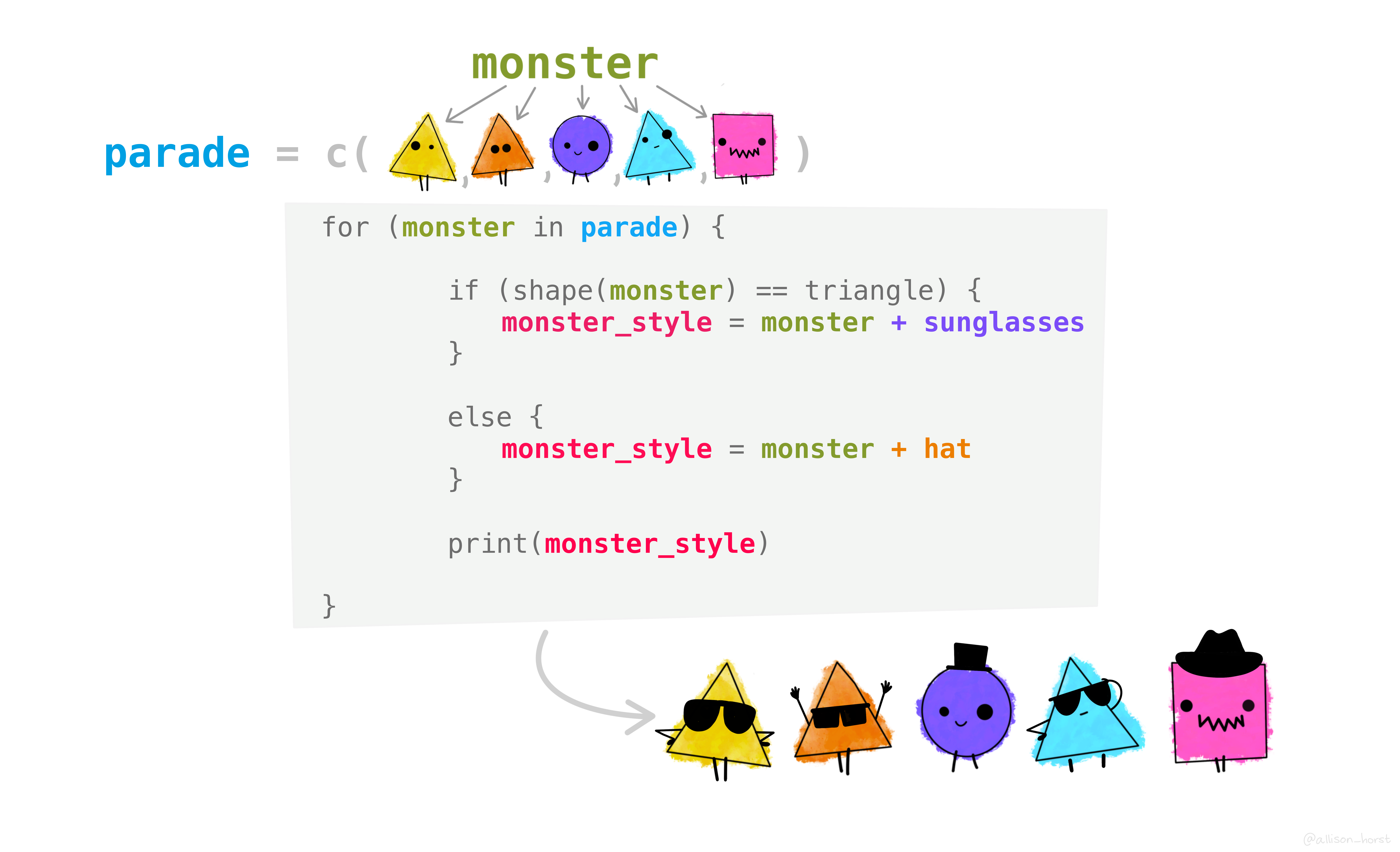
Illustrated for loop example. Input vector is a parade of monsters, including monsters that are circles, triangles, and squares. The for loop they enter has an if-else statement: if the monster is a triangle, it gets sunglasses. Otherwise, it gets a hat. The output is the parade of monsters where the same input parade of monsters shows up, now wearing either sunglasses (if triangular) or a hat (if any other shape).

Conditional Statements

Conditional statements allow you to execute different blocks of code based on whether certain conditions are met.

Statement Description
if Execute a block of code if a specified condition is TRUE
if...else Execute one block of code if a condition is TRUE,
if...else if...else Execute different blocks of code based on multiple conditions
# if statement

x <- 3

if (x > 0) {
    print("x is positive")
}
[1] "x is positive"
# if...else statement
y <- 10

if (y > 5) {
    print("y is greater than 5")
} else {
    print("y is not greater than 5")
}
[1] "y is greater than 5"

Conditional Statements: Example

# Example of if...else if...else statement

z <- 0 # change this value to test different outcomes

# Check if z is a number
# if it is, do the checks inside the {}
# if it isn't, go to the else statement
if (is.numeric(z)) {
    if (z > 0) {      # is it positive?
        print("z is positive")  # if it is, say so and then STOP
    # if not, is it negative?
    } else if (z < 0) {     # if not, is it negative?
        # if it is, say so and then STOP
        print("z is negative")  # if it is, say so and then STOP
    # if not positive and not negative, it must be zero
    } else {
        print("z is zero") # say so and then STOP
    }
# if it isn't a number, say so and then STOP
} else {
    print("z is not a number")
}
[1] "z is zero"

Conditional Functions

R’s conditional functions provide a way to perform conditional operations in a more functional, condensed style.

Function Package
ifelse() base
if_else() dplyr
case_when() dplyr

The examples from the previous slide can be written more concisely:

y <- 10

ifelse(y > 5, "y is greater than 5", "y is not greater than 5")
[1] "y is greater than 5"
z <- 0 # change this value to test different outcomes

print(case_when(
    !is.numeric(z) ~ "z is not a number",
    z > 0 ~ "z is positive",
    z < 0 ~ "z is negative",
    TRUE ~ "z is zero"
))
[1] "z is zero"

Iteration

Iteration, or looping, allows you to repeat a block of code multiple times, either a fixed number of times or while a certain condition is met.

Loop Type Description
for Repeats a block of code for each item in a sequence or vector
while Repeats a block of code as long as a specified condition is TRUE

Loops Conceptually

When I say go

Do this thing

And keep doing it

Until I say stop

for Loops

When I say go

i = my_list[1]

Do this thing

print(i)

And keep doing it

i = my_list[2]
i = my_list[3]...

Until I say stop

my_list[6] > length(my_list)

# Create a finite sequence of numbers
my_list <- c(1, 3, 5, 7, 9)

# for each value i in the sequence num_list
for (i in my_list) {
    # print the value of i to the console
    print(i)
# iterate to the next value in the sequence 
    # until there are no values left
}
[1] 1
[1] 3
[1] 5
[1] 7
[1] 9

while Loops

When I say go

i = 1

Do this thing

print(i)
i <- i + 1

And keep doing it

print(i + 1)
print(i + 2)...

Until I say stop

i >= 6

# Initialize counter variable i to 1
i <- 1 

# while (if) i=1, then i=2...til i=6
while (i < 6) {
    # print the value of i to the console
    print(i)
    i <- i + 1 # Increment i by 1
# check whether "while" condition still holds
    # repeat if TRUE
    # stop if FALSE
}
[1] 1
[1] 2
[1] 3
[1] 4
[1] 5

for vs while

for

  • Known, finite sequence
  • Repeats for each item in sequence
  • Does not require an explicit counter variable
  • Iteration happens automatically

while

  • Unknown, potentially infinite sequence
  • Repeats while condition is TRUE
  • Requires an explicit counter variable
  • Iteration controlled by defined condition

Warning: Infinite loops

Use while for potentially but not actually infinite sequences. Your code must eventually lead to a FALSE evaluation:

  1. Define the iteration mechanism:
    • i <- i+1
  2. Ensure the while condition will eventually be FALSE when iterated using that mechanism
    • i < 6

Regular Expressions

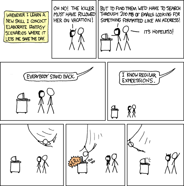
xkcd comic strip about regular expressions. Two people are lamenting having to find text formatted as an email address. A third character swoops in on a rope saying 'Everybody stand back. I know regular expressions.', types something, and swoops away.

What are Regular Expressions?

Regular expressions (regex or regexp): sequences of characters that form a search pattern, primarily used for string matching and manipulation.

Examples of regex syntax:

  • ^Hello: matches any string that starts with “Hello”
  • [aeiou]: matches any single vowel character (a, e, i, o, u)
  • \d{3}-\d{2}-\d{4}: matches a pattern like a US Social Security number (e.g., “123-45-6789”)
    • or with R’s escaping: \\d{3}-\\d{2}-\\d{4}

Tip

Use tools like regex101 or RegExr to test and visualize regex patterns interactively. Just be careful about escaping rules when using R! (More info below.)

Basic Regex Syntax: Essentials

Symbol Description Example
. Matches any single character except newline a.b matches “acb”, “a1b”, “a b”
^ Matches the start of a string ^Hello matches “Hello world”
$ Matches the end of a string world$ matches “Hello world”
* Matches 0 or more occurrences of the preceding element ab* matches “a”, “ab”, “abb”, “abbb”
+ Matches 1 or more occurrences of the preceding element ab+ matches “ab”, “abb”, “abbb” but not “a”
? Matches 0 or 1 occurrence of the preceding element ab? matches “a” and “ab”
[] Matches any one character within the brackets [aeiou] matches “a”, “e”, “i”, “o”, or “u”
| Logical OR operator cat|dog matches “cat” or “dog”
() Groups expressions (ab)+ matches “ab”, “abab”, “ababab”

Basic Regex Syntax: Other Useful Matches

Symbol Description Example
\d Matches any digit (0-9) \d matches “0”, “1”, …, “9”
\w Matches any word character (alphanumeric + underscore) \w matches “a”, “b”, …, “z”, “A”, “B”, …, “Z”, “0”, “1”, …, “9”, “_”
\s Matches any whitespace character (space, tab, newline) \s matches ” “,”, “”
{n} Matches exactly n occurrences of the preceding element a{3} matches “aaa”
{n,} Matches n or more occurrences of the preceding element a{2,} matches “aa”, “aaa”, “aaaa”, …
{n,m} Matches between n and m occurrences of the preceding element a{2,4} matches “aa”, “aaa”, or “aaaa”

Escaping

Characters that have assigned functions will perform that function unless they are escaped.

Escape a special character to refer to its literal meaning.

  • R uses a backslash (\) as the escape character.
  • Regex also uses a backslash (\) as the escape character.
  • When using regex in R, you need to use double backslashes (\\) to escape special characters because the backslash itself is an escape character in R strings.

TELL ME WHY.

Using Regex in R (with base)

Base R uses “grep” functions for regex operations.

  • grep = global regular expression print.
  • Semi-consistent argument order: function_name(pattern_to_find, string_to_search, other_args)

Common grep functions:

  • grep(): Search for patterns in strings and return indices of matches
  • grepl(): Search for patterns and return logical vector indicating matches
  • gsub(): Replace occurrences of a pattern with a specified replacement

Using Regex in R (with base): Examples

# Example strings
text <- "The rain in Spain stays mainly in the plain."
title <- "My Fair Lady"
# Find which list elements contain "ain"
grep("ain", c(title, text))
[1] 2
# Replace "ain" with "XXX"
gsub("ain", "XXX", text)
[1] "The rXXX in SpXXX stays mXXXly in the plXXX."
# Check if the string starts with "The"
grepl("^The", text)
[1] TRUE

Using Regex in R (with stringr)

The stringr package (part of the tidyverse) provides an alternative set of string manipulation functions, using consistent syntax and behavior across nearly all stringr functions

  • Naming: str_ + descriptive function name
  • Argument order: str_func(string_to_search, pattern_to_find, other_args)
    • Note: this flips the order of the first two arguments compared to base R’s grep functions
  • Accepts regex patterns plus some user-friendlier, tidyvers-ier enhancements

Common stringr functions:

  • str_which(): Search for patterns in strings and return indices of matches
  • str_detect(): Search for patterns and return logical vector indicating matches
  • str_replace_all(): Replace occurrences of a pattern with a specified replacement

Using Regex in R (with stringr): Examples

# Load stringr package for string manipulation
library(stringr)

# Example strings
text <- "The rain in Spain stays mainly in the plain."
title <- "My Fair Lady"
# Find which list elements contain "ain"
str_which(c(title, text), "ain")
[1] 2
# Replace "ain" with "XXX"
str_replace_all(text, "ain", "XXX")
[1] "The rXXX in SpXXX stays mXXXly in the plXXX."
# Check if the string starts with "The"
str_detect(text, "^The")
[1] TRUE

Summary

R Language

  • R is an object-oriented programming language for statistical computing and graphics
  • R syntax includes:
    • Variables: store data values
    • Data Types: numeric, character, logical, etc.
    • Data Structures: vectors, lists, data frames, matrices
    • Functions: reusable blocks of code that perform specific tasks
    • Comments: annotate code with #, ignored by R
  • Case-sensitive but whitespace insensitive
  • Functions are called using parentheses, with arguments passed inside
  • Install and load packages to extend R’s functionality with additional functions and tools

R Programming

  • Indexing and Subsetting: selecting specific elements from data structures using position or name
  • Environments: data structures that store scoped variable bindings, including global and local environments
  • Control Flow: managing the order of code execution using
    • Conditional statements (if, if...else)
    • Conditional functions (ifelse(), case_when())
    • for loops: iterate over a known, finite sequence
    • while loops: iterate while a condition is TRUE
  • Regular Expressions (regex): sequences of characters forming search patterns for string matching and manipulation
    • Basic syntax includes symbols like ., ^, $, *, +, ?, [], |, ()
    • Escaping special characters with backslashes (\), using double backslashes (\\) in R strings
    • Use regex in R with base grep-style functions or stringr str_-style functions