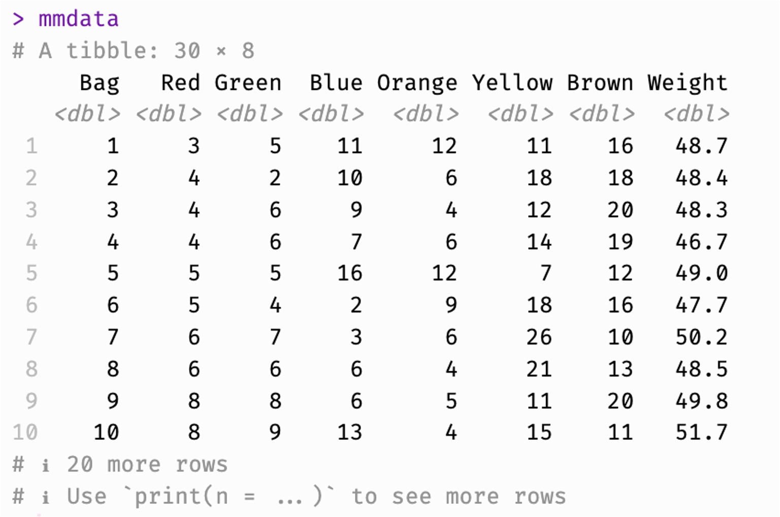
Welcome to the Tidyverse

ecosystem, read-in/-out, data manipulation

2026-01-27

Tidy Data

What Makes Data “Tidy”?

Illustrations from the Openscapes blog Tidy Data for reproducibility, efficiency, and collaboration by Julia Lowndes and Allison Horst

Messy vs. Tidy: Example

These tables hold exactly the same data!

What are the differences? What are the advantages of each?

mm.raw

# A tibble: 30 × 8
     Bag   Red Green  Blue Orange Yellow Brown Weight
   <int> <dbl> <dbl> <dbl>  <dbl>  <dbl> <dbl>  <dbl>
 1     1    15     9     3      3      9    19   49.8
 2     2     9    17    19      3      3     8   49.0
 3     3    14     8     6      8     19     4   50.4
 4     4    15     7     3      8     16     8   49.2
 5     5    10     3     7      9     22     4   47.6
 6     6    12     7     6      5     17    11   49.8
 7     7     6     7     3      6     26    10   50.2
 8     8    14    11     4      1     14    17   51.7
 9     9     4     2    10      6     18    18   48.4
10    10     9     9     3      9      8    15   46.2
# ℹ 20 more rows

mm.tidy

# A tibble: 180 × 4
     Bag Color  Number Bag_Weight
   <int> <chr>   <dbl>      <dbl>
 1     1 Red        15       49.8
 2     1 Green       9       49.8
 3     1 Blue        3       49.8
 4     1 Orange      3       49.8
 5     1 Yellow      9       49.8
 6     1 Brown      19       49.8
 7     2 Red         9       49.0
 8     2 Green      17       49.0
 9     2 Blue       19       49.0
10     2 Orange      3       49.0
# ℹ 170 more rows

That messy data looks pretty clean to me…

It is clean! It’s just not tidy.

Terminology Detour

Messy, Clean, Tidy

Messy data:

mm.raw

# A tibble: 30 × 8
     Bag   Red Green  Blue Orange Yellow Brown Weight
   <int> <dbl> <dbl> <dbl>  <dbl>  <dbl> <dbl>  <dbl>
 1     1    15     9     3      3      9    19   49.8
 2     2     9    17    19      3      3     8   49.0
 3     3    14     8     6      8     19     4   50.4
 4     4    15     7     3      8     16     8   49.2
 5     5    10     3     7      9     22     4   47.6
 6     6    12     7     6      5     17    11   49.8
 7     7     6     7     3      6     26    10   50.2
 8     8    14    11     4      1     14    17   51.7
 9     9     4     2    10      6     18    18   48.4
10    10     9     9     3      9      8    15   46.2
# ℹ 20 more rows

Also messy data:

mm.messy

# A tibble: 39 × 8
   ID    RED   X     GREEN WT.GRAM  Blue  Orannge Ylw. 
   <chr> <chr> <chr> <chr> <chr>    <chr> <chr>   <chr>
 1 "1 "  "15"  "19 " "9 "  "49.79 " "3 "  "3 "    "9 " 
 2 "1 "  "15"  "19 " "9 "  "49.79 " "3 "  "3 "    "9 " 
 3 "2 "  "9"   "8 "  "17 " "48.98 " "19 " <NA>    "3 " 
 4 "3 "   <NA> "4 "  "8 "  "50.4 "  "6 "  "8 "    "19 "
 5 "4 "  "15 " "8 "  "7 "  "49.16 "  <NA> "8 "    "16 "
 6 "5"   "10 " "4 "  "3 "  "47.61 " "7 "  <NA>     <NA>
 7 "6 "  "12 " "11 " "7 "  "49.8"   "6 "  "5 "    "17 "
 8 "7 "  "6 "  "10 " "7 "  "50.23 " "3 "  "6 "    "26 "
 9 "8 "  "14 " "17 " "11 " "51.68 " "4 "  <NA>    "14 "
10 "8 "   <NA> "17 " "11 " "51.68 " "4 "  "1 "    "14 "
# ℹ 29 more rows

messy ≠ bad (except in the tidyverse context)

• Data wrangling starts with reading your data, then prepping it for visualization & analysis
• To use tidyverse packages, this prepping includes tidying messy data
• This can be shockingly complicated and time-consuming!

“Messy” is messy

Messy can either mean “not clean” or “not tidy”

• Always bad: unclean + untidy (= messy)
• Sometimes good: clean + untidy (= messy)
• Usually good: clean + tidy (= tidy)

It would make more sense to call it “untidy.”

You are not wrong.

Tidy Data: Iris

The iris dataset is a classic example of tidy data.

Which of these two versions of iris is tidy?

In tidy data:

1. Each variable is one column.
2. Each observation is one row.
3. Each measurement is one cell.
4. Each unit depends on the research question.

iris_1

   Sepal.Length Sepal.Width Petal.Length Petal.Width Species
1           5.1         3.5          1.4         0.2  setosa
2           4.9         3.0          1.4         0.2  setosa
3           4.7         3.2          1.3         0.2  setosa
4           4.6         3.1          1.5         0.2  setosa
5           5.0         3.6          1.4         0.2  setosa
6           5.4         3.9          1.7         0.4  setosa
7           4.6         3.4          1.4         0.3  setosa
8           5.0         3.4          1.5         0.2  setosa
9           4.4         2.9          1.4         0.2  setosa
10          4.9         3.1          1.5         0.1  setosa

iris_2

# A tibble: 10 × 4
   Species Flower_Part Measurement_Type value
   <fct>   <chr>       <chr>            <dbl>
 1 setosa  Sepal       Length             5.1
 2 setosa  Sepal       Width              3.5
 3 setosa  Petal       Length             1.4
 4 setosa  Petal       Width              0.2
 5 setosa  Sepal       Length             4.9
 6 setosa  Sepal       Width              3  
 7 setosa  Petal       Length             1.4
 8 setosa  Petal       Width              0.2
 9 setosa  Sepal       Length             4.7
10 setosa  Sepal       Width              3.2

Consider iris—each row is one flower with four morphological measurements (sepal length, sepal width, petal length, petal width). This is tidy for the question: “What morphological features distinguish these species?”

Could you pivot iris longer with columns for flower_part (sepal/petal) and measurement_type (length/width)? Yes. Would it be tidy? Also yes—but for a different question: “What determines the size of flower parts in general?”

The key distinction: Are your columns measuring different variables or different levels of the same variable?

• Different variables → Keep separate columns
• Different levels → Pivot longer

Tidiness isn’t absolute. It’s defined by your analytical question. The same dataset can be tidy in multiple forms depending on what you’re studying.

Data Preparation Terms

Process	Start State	Goal	End State	Examples
Data Cleaning: Error correction	Raw data	Accuracy, consistency, legibility	Clean data, not yet specialized	Removing duplicate data Correcting syntax errors Fixing typos Handling missing values Change data types
Data Wrangling: Data preparation	Clean data	Usability for medium-scope purpose	Interpretable and specialized data, not yet analyzable	Preparing for narrow use cases Grouping and summarizing Transforming variables or values
Data Transformation: Data restructuring	Interpretable data	Usability for narrow-scope tasks	Analyzable and visualizable data	Reshaping long ↔︎ wide Generating new data-based variables Merging datasets Eliminating unnecessary data

You use them differently in the core project instructions!

Those are the same thing!

That’s not what I learned!

OK FINE. Yes. You’re all correct. You’re also all incorrect. Honestly it doesn’t really matter. Just mess with your data until they are usable. Call it what you want as long as it works.

Tidyverse Packages

tibble

Reimagine the dataframe

readr

import and export tabular data

dplyr

a grammar of data manipulation

tidyr

tidy your messy data

purrr

enhance R’s functional programming

stringr

simplify working with strings

forcats

simplify working with factors

ggplot2

a grammar of graphics

tibble

tibble: Better Data Frames

)

tibble:
Better data frames

• Adaptation of base R’s data.frame
• Tibbles are also data.frames
  • Check with class() or str()
• Tidyverse functions work with tibbles
  • usually add the tibble class automatically
• Functionally equivalent

Adaptation of base R’s data.frame structure that makes a lot of things easier Tibbles are also data.frames (check the class() or str() functions) Tidyverse package(s) work with tibbles, not base data.frames Load the tidyverse library to use tibble-related functions

tibble: implicit data

• Most Tidyverse functions take and return tibbles
  • Notably dplyr, tidyr, and ggplot2
  • Tibble is the required first argument (i.e., data)
• As standalone functions, these require an explicit tibble argument:
  • 1st arg: function(my_tbl, arg1, arg2)
  • Anywhere: function(arg1, arg2, data = my_tbl)
• In pipelines using (%>% or |>), the tibble is implicit (omitted)
  • Tibble output from function1() pipes |> to tibble input for function2()
  • function1(data, arg1, arg2) %>% function2(arg1, arg2)

More on pipes later

More on the pipe operator and pipelines later. For now, know that when these slides show non-executed examples as function(arg1, arg2) as shorthand for function(data, arg1, arg2).

The first argument for most tidyverse functions is data, the tbl passed to the function.

When running a tidyverse function on its own, you must include the tibble explicitly as a required argument either unnamed in the first position (function(my_tbl, arg1, arg2)) or anywhere by name (function(arg1, arg2, data = my_tbl)).

However, tidyverse functions are often used in a pipeline where the tibble is passed from one function to the next using a pipe operator (%>% or |>). Since tidyverse functions both take and return a tibble, the pipe automatically passes the output of one function as the first argument (data) of the next function in the chain, letting you omit it.

More on the pipe later. For now, know that when these slides show non-executed examples as function(arg1, arg2) as shorthand for function(data, arg1, arg2).

readr

readr: Read & Write Tibbles

)

readr:
Read & Write Tibbles

• Import/export tabular data as tibbles
• Functions start with read_*() and write_*()
• Handle common file types: CSV, TSV, delimited, fixed-width
• Other packages for Excel, SPSS, Google Sheets, JSON, databases

What & Where

Determine import function:

• File extension?
• Field separators?
• Column names?
• Non-tabular content?
• Multiple sheets?

Determine file path:

• Located in your repo
• Protected data
  • Add to .gitignore or localonly
  • Only call in your local R scripts
• Shared data
  • In git-managed directory
  • Callable by any/all scripts
• Use relative paths

Relative relativity

Quarto documents handle relative paths differently than R scripts.

In scripts, relative paths are relative to the working directory, your repo or project’s top-level. In Quarto docs, relative paths are relative to the location of the Quarto file itself.

If you work in a single .qmd in the top-level of your repo, these are equivalent. Read from: repo_name/data/file.csv

If your .qmd is in any subfolder, you’ll need to adjust. To read the same file from a code chunk in repo_name/quarto/document.qmd, use: ../data/file.csv

This is for all file operations, not just readr functions.

readr cheatsheet

Importing with readr

)

Importing with readr: read_*()

• read_*() import tabular data as tibbles
• Optional col_types & col_names arguments:
• Assign to object to save imported data

# Common read functions

read_csv()    # Comma separated values
read_csv2()   # Semicolon separator (comma = decimal)
read_tsv()    # Tab separated values
read_delim()  # Any delimiter
read_fwf()    # Fixed width files
read_table()  # Whitespace separated

# Default behavior - guesses all data types
my_tbl <- read_*(file.csv, col_types = NULL)

# Specify columns with cols()
my_cols <- read_*(file.csv, col_types = cols(
  my_factor = col_factor(),
  your_string = col_character()
))

# String shortcut:
# needs character for each col in order
# Use "?" for columns to guess
my_shortcut <- read_*(file.csv, col_types = "fc")

Exporting with readr

)

Exporting with readr: write_*()

• read_*() functions have matched write_*() counterparts
• Save tibbles to tabular files
• Write intermediate datasets after:
  • De-identifying data
  • Complex wrangling
  • Dropping unneeded data
  • Managing empty data
• Run from script or console, no object assignment

# Common write_*() functions

write_delim()
write_csv()
write_csv2()
write_excel_csv()
write_excel_csv2()
write_tsv()

# Start with messy data
messy_df <- read_xlsx("localpath/messy.xlsx", 
                     sheet="my sheet")

# Process in R: tidy, clean, transform...

# Export clean version
clean_df <- # ... your cleaning steps
write_csv(clean_df, "localpath/clean.csv")

# Later, read the clean version
clean_df <- read_csv("localpath/clean.csv")

Export tibbles to create intermediate datasets between initial import and final analysis Easily produce de-identified datasets to share with others Save computational time by skipping costly read-in and wrangling steps (e.g., big files, many files, complex transformations) readr can also export tibbles to tabular files with similar syntax to how it imports

# Read in messy data
messy_df <- read_xlsx(
    "localpath/messy.xlsx",
    sheet="my sheet"
    )

.

My tidy data file:

• Data needed for future R scripts and nothing else
• Minimal, tabular (.csv)
• No protected data
• Added variables from initial wrangling

# Write out clean version
write_csv(clean_df, 
          "localpath/clean.csv")

# Read in clean version
clean_df <- read_csv(
    "localpath/clean.csv")

clean_df:

• Clean & tidy tibble
• Data needed for analysis and nothing else

Bonus: readxl & googlesheets4

Complementary packages to readr

• Mimic readr’s read_* functions
  • same cheatsheet
• Specification for converting “complex” documents into a tbl-compatible format
• Not tidyverse packages
  • Install and load them separately!

# readxl for Excel files
library(readxl)
read_excel("data.xlsx")

# googlesheets4 for Google Sheets
library(googlesheets4)
read_sheet("spreadsheet_url")

Practice: Read & Write (1)

Read in M&M data:

1. Pull the student-hub repo (or find files on GitHub)
2. Find the Excel spreadsheet: data/MM data.xlsx
3. Install and load the readxl library
4. Use the read_excel() function to assign the data to a tibble called mmdata
5. Examine your data in the console to see if it matches the image

It doesn’t!

Oh no! Thank heavens you are smarter than a computer.

Practice: Read & Write (2)

Fix, read, write:

1. Open MM data.xlsx in Excel (or similar) and examine it with your human eyeballs
   • What about this file creates problems when you read-in?
   • How might you fix the issue here in the Excel document?
2. Review the ?read_excel documentation
   • What arguments can you pass to read_excel() to fix the issue on read-in?
3. Use read_excel() to assign the data to a tibble called mmdata that looks like the image
4. Use write_csv() to save mmdata to an intermediate dataset at the location student-hub/data/mmdata.csv
   • Use an appropriate relative path!

It says that folder doesn’t exist!
(and/or)
It doesn’t read/write/both where I want it to!

Remember relative relativity. Are you reading and writing from a script, Quarto doc, or the console?

Open MM data.xlsx in Excel (or similar) and examine it with your human eyeballs What about this file creates problems when you read-in? How would you fix the issue here in the Excel document? (just think; don’t do it!) Review the ?read_excel documentation What arguments can you pass to read_excel() to fix the issue on read-in? Use the read_excel() function to assign the data to a tibble called mmdata that looks like the image Use write_csv() to save mmdata to an intermediate dataset: in-class-materials/data/mmdata.csv

dplyr

dplyr: Data Transformation

dplyr:
Grammar of Data Manipulation

• Core tidyverse package for data transformation
• Works with tibbles (and data.frames)
• First argument always data (the tibble to transform)

select

subset & sort columns

filter

subset rows

arrange

sort rows

mutate

create and modify columns

summarize

compute with multiple rows

group_by

perform operations on subgroups

select: Subset columns

Include/exclude syntax:

select(tbl, col1, col2, ...)

• Column names are objects, not strings
  • select(mm.sample, Bag, Red)
  • not select(mm.sample, "Bag", "Red")

• Include (default):
  • select(col1, col2)

• Exclude with -:
  • select(-col3, -col4)
  • select(-c(col3, col4))

• Use ranges:
  • Name: select(colA:colC)
  • Position: select(1:3)
  • Exclude: select(-(4:6))

# Include specific columns 
select(mm.sample, Bag, Red, Green, Blue)

# Exclude specific columns
select(mm.sample, -Orange, -Yellow, -Brown, -Weight)

# Exclude list of columns
select(mm.sample, -c(Orange, Yellow, Brown, Weight))

# Include columns by name range
select(mm.sample, Bag:Blue)

# Exclude columns by position range
## `-` requires range in `()`
select(mm.sample, -(5:8))

# A tibble: 5 × 4
    Bag   Red Green  Blue
  <int> <dbl> <dbl> <dbl>
1     1    15     9     3
2     2     9    17    19
3     3    14     8     6
4     4    15     7     3
5     5    10     3     7

select: Rename & reorder columns

Rename & order:

• Select & reorder:
  • select(col3, col1, col2)

• Select & rename:
  • select(new_name = old_name)

• Backticks for special characters:
  • select(`col 2 (two)` = col2)

• Related function: rename()
  • Rename some or all columns
  • Retain all columns in original order

• Related function: relocate()
  • Move columns to relative positions
  • relocate(col3, .before = col1)
  • Retain all columns in original order

# Select and reorder
select(mm.sample, 
       Green, Blue, Bag, Red)

# A tibble: 5 × 4
  Green  Blue   Bag   Red
  <dbl> <dbl> <int> <dbl>
1     9     3     1    15
2    17    19     2     9
3     8     6     3    14
4     7     3     4    15
5     3     7     5    10

# Select and rename
select(mm.sample, 
       Bag, rojo = Red, 
       vert = Green, 
       `aoi 青` = Blue)

# A tibble: 5 × 4
    Bag  rojo  vert `aoi 青`
  <int> <dbl> <dbl>    <dbl>
1     1    15     9        3
2     2     9    17       19
3     3    14     8        6
4     4    15     7        3
5     5    10     3        7

# Select, reorder, rename
select(mm.sample, 
       vert = Green, 
       rojo = Red, 
       `aoi 青` = Blue, 
       Bag)

# A tibble: 5 × 4
   vert  rojo `aoi 青`   Bag
  <dbl> <dbl>    <dbl> <int>
1     9    15        3     1
2    17     9       19     2
3     8    14        6     3
4     7    15        3     4
5     3    10        7     5

# Rename w/out select or reorder
rename(mm.sample, 
       vert = Green, 
       rojo = Red, 
       `aoi 青` = Blue)

# A tibble: 5 × 8
    Bag  rojo  vert `aoi 青` Orange Yellow Brown Weight
  <int> <dbl> <dbl>    <dbl>  <dbl>  <dbl> <dbl>  <dbl>
1     1    15     9        3      3      9    19   49.8
2     2     9    17       19      3      3     8   49.0
3     3    14     8        6      8     19     4   50.4
4     4    15     7        3      8     16     8   49.2
5     5    10     3        7      9     22     4   47.6

select Helpers

tidy-select

• starts_with("prefix")

• ends_with("suffix")

• contains("text")

• matches("regex")

• num_range("x", 1:5)

• everything()

# Select by first character(s)
select(mm.sample, 
       starts_with("B"))

# A tibble: 5 × 3
    Bag  Blue Brown
  <int> <dbl> <dbl>
1     1     3    19
2     2    19     8
3     3     6     4
4     4     3     8
5     5     7     4

# Select by last character(s)
select(mm.sample, 
       ends_with("n"))

# A tibble: 5 × 2
  Green Brown
  <dbl> <dbl>
1     9    19
2    17     8
3     8     4
4     7     8
5     3     4

# Select with regex
select(mm.sample, 
       contains("ow"))

# A tibble: 5 × 2
  Yellow Brown
   <dbl> <dbl>
1      9    19
2      3     8
3     19     4
4     16     8
5     22     4

# Select with regex
select(mm.sample, 
       matches("^B|n$"))

# A tibble: 5 × 4
    Bag Green  Blue Brown
  <int> <dbl> <dbl> <dbl>
1     1     9     3    19
2     2    17    19     8
3     3     8     6     4
4     4     7     3     8
5     5     3     7     4

Operates on columns/variables (not observations/rows) Returns a tibble with only the given columns in the order given renamed if provided Remove columns with the hyphen Includes everything not explicitly mentioned Rename as you select with new_name = old_name

filter: Subset rows

Filter syntax & logic:

filter(tbl, cond1, cond2, ...)

• Operates on rows (observations)
• Conditional evaluation:
  • Comparison operators (e.g., >, !=, ==)
  • Logical operators (e.g., &, |, !)
  • Boolean values (TRUE, FALSE)
• Returns tibble with rows that meet all conditions

# Vehicle dataframe (1 column called `transport`)
vehicles <- data.frame(
    transport = c("walking", "bus", "bicycle", "car", "atv",
                   "motorcycle", "razor scooter", "the el", 
                   "jet ski", "sailboat", "tricycle", "chariot"))

# Condition 1
filter(vehicles, transport == "bicycle")

# Condition 2
filter(vehicles, 
       has.handlebars(transport) | transport == "boat")

# Condition 3
filter(vehicles, 
       has.handlebars(transport), transport == "boat")

# Condition 3
filter(vehicles, 
       (has.handlebars(transport) & n.wheels(transport) < 3) |
           (requires.gas(transport) & n.wheels(transport) > 3))

Condition 1:

  transport
1   bicycle

Condition 2:

      transport
1       bicycle
2           atv
3    motorcycle
4 razor scooter
5       jet ski

Condition 3:

[1] transport
<0 rows> (or 0-length row.names)

Condition 4:

      transport
1           bus
2       bicycle
3           car
4    motorcycle
5 razor scooter
6       jet ski

Operates on observations/rows (not columns!) Conditions are logical evaluations using: >, >=, <, <=, != (“not equal to”), and == (“equal to”) If the condition evaluates to TRUE, it stays and is returned or passed to the next line of the pipe If FALSE, it’s filtered out

filter: Subset rows

Filter example:

# Condition 1
filter(mm.tidy, Bag_Weight > 50)

# Condition 2
filter(mm.tidy, 
       Color == "Red" | Number >= 15)

# Condition 3
filter(mm.tidy, 
       Color == "Red", Number >= 15)

# Condition 4
filter(mm.tidy, 
       (Color == "Blue" & Number >= 5) |
           (Bag_Weight > 50.5 | Bag_Weight < 47),
       Bag != 6)

Condition 1:

# A tibble: 54 × 4
     Bag Color  Number Bag_Weight
   <int> <chr>   <dbl>      <dbl>
 1     3 Red        14       50.4
 2     3 Green       8       50.4
 3     3 Blue        6       50.4
 4     3 Orange      8       50.4
 5     3 Yellow     19       50.4
 6     3 Brown       4       50.4
 7     7 Red         6       50.2
 8     7 Green       7       50.2
 9     7 Blue        3       50.2
10     7 Orange      6       50.2
# ℹ 44 more rows

Condition 2:

# A tibble: 58 × 4
     Bag Color  Number Bag_Weight
   <int> <chr>   <dbl>      <dbl>
 1     1 Red        15       49.8
 2     1 Brown      19       49.8
 3     2 Red         9       49.0
 4     2 Green      17       49.0
 5     2 Blue       19       49.0
 6     3 Red        14       50.4
 7     3 Yellow     19       50.4
 8     4 Red        15       49.2
 9     4 Yellow     16       49.2
10     5 Red        10       47.6
# ℹ 48 more rows

Condition 3:

# A tibble: 4 × 4
    Bag Color Number Bag_Weight
  <int> <chr>  <dbl>      <dbl>
1     1 Red       15       49.8
2     4 Red       15       49.2
3    23 Red       20       50.0
4    29 Red       15       49.4

Condition 4:

# A tibble: 62 × 4
     Bag Color  Number Bag_Weight
   <int> <chr>   <dbl>      <dbl>
 1     2 Blue       19       49.0
 2     3 Blue        6       50.4
 3     5 Blue        7       47.6
 4     8 Red        14       51.7
 5     8 Green      11       51.7
 6     8 Blue        4       51.7
 7     8 Orange      1       51.7
 8     8 Yellow     14       51.7
 9     8 Brown      17       51.7
10     9 Blue       10       48.4
# ℹ 52 more rows

Operates on observations/rows (not columns!) Conditions are logical evaluations using: >, >=, <, <=, !=, == If the condition evaluates to TRUE, it stays and is returned or passed to the next line of the pipe If FALSE, it’s filtered out

arrange: Sort rows

Arrange syntax:

arrange(tbl, col1, col2, ...)

• Sort rows by column values
• If 2+ variables, sorts in order given
• Strings sorted alphabetically
• Ascending order (default)
• Descending order:
  • arrange(desc(col1))
  • arrange(-col1)

# Sort by (ascending) bag weight
arrange(mm.tidy, Bag_Weight)

# A tibble: 180 × 4
     Bag Color  Number Bag_Weight
   <int> <chr>   <dbl>      <dbl>
 1    10 Red         9       46.2
 2    10 Green       9       46.2
 3    10 Blue        3       46.2
 4    10 Orange      9       46.2
 5    10 Yellow      8       46.2
 6    10 Brown      15       46.2
 7    26 Red         4       46.7
 8    26 Green       6       46.7
 9    26 Blue        7       46.7
10    26 Orange      6       46.7
# ℹ 170 more rows

# Sort by color -> desc number -> desc bag
arrange(mm.tidy, Color, -Number, desc(Bag))

# A tibble: 180 × 4
     Bag Color Number Bag_Weight
   <int> <chr>  <dbl>      <dbl>
 1     2 Blue      19       49.0
 2    19 Blue      16       49.0
 3    20 Blue      13       51.7
 4    13 Blue      13       46.9
 5    11 Blue      13       50.4
 6    27 Blue      11       47.7
 7    17 Blue      11       48.7
 8     9 Blue      10       48.4
 9    16 Blue       9       48.3
10    30 Blue       7       52.1
# ℹ 170 more rows

Sort rows of your tibble in the order of col1, then col2, etc. Defaults to ascending order, but you can wrap the column name in the desc() function to use descending order The hyphen - is shorthand for desc()

mutate: Create & modify columns

Create & modify:

mutate(tbl, 
    new_col1 = ..., 
    new_col2 = ..., 
    ...)

• Add named new column
• Assign values with =
• Compute values by row
• Columns created in order
  • Reference a newly created column in subsequent columns
• Modify an existing column by creating a new column with the same name

# Create new column: Weight_Oz
# then pipe to select cols
mutate(mm.sample,
    Type = "Chocolate") |> 
    select(Bag, Weight, Type) 

# A tibble: 5 × 3
    Bag Weight Type     
  <int>  <dbl> <chr>    
1     1   49.8 Chocolate
2     2   49.0 Chocolate
3     3   50.4 Chocolate
4     4   49.2 Chocolate
5     5   47.6 Chocolate

# Create new column: Weight_Oz
mutate(mm.sample,
    Weight_Oz = Weight / 28.34952) |> 
    select(Bag, Weight, Weight_Oz)

# A tibble: 5 × 3
    Bag Weight Weight_Oz
  <int>  <dbl>     <dbl>
1     1   49.8      1.76
2     2   49.0      1.73
3     3   50.4      1.78
4     4   49.2      1.73
5     5   47.6      1.68

# Create new column (total M&Ms per bag)
# Then another new column (proportion of red M&Ms)
# using the first new column
mutate(mm.sample,
    Total_MMs = Red + Green + Blue + 
        Brown + Yellow + Orange,
        Prop_Red = Red / Total_MMs) |> 
    select(Bag, Red, Total_MMs, Prop_Red)

# A tibble: 5 × 4
    Bag   Red Total_MMs Prop_Red
  <int> <dbl>     <dbl>    <dbl>
1     1    15        58    0.259
2     2     9        59    0.153
3     3    14        59    0.237
4     4    15        57    0.263
5     5    10        55    0.182

# Change values in existing column by overwriting
mutate(mm.sample,
        Weight = case_when(
        Weight < 48 ~ "Light",
        Weight > 50 ~ "Heavy",
        TRUE ~ "Medium" # anything left after
        )) |> 
select(Bag, Red, Weight)

# A tibble: 5 × 3
    Bag   Red Weight
  <int> <dbl> <chr> 
1     1    15 Medium
2     2     9 Medium
3     3    14 Heavy 
4     4    15 Medium
5     5    10 Light 

Adds new column(s) with names and values that you define Use the single equals sign to assign new values Use double equal signs to mean “equals” within a conditional statement *Use mutate to effectively change data in an existing variable by creating a new variable with the same name that will overwrite it

summarize & group_by: Compute summary values

Group & summarize:

group_by(tbl, col1, col2, ...)  |> 
summarize(
    summary_col1 = summary_func(colA),
    summary_col2 = summary_func(colB),
...)

• group_by() creates subgroups based on unique values across 1+ columns
  • Tidy grouping needs tidy data
• summarize() computes summary functions across those groups
  • e.g., mean(), max(), last(), n()
• Output tibble includes:
  • Grouping column(s)
  • New summary column(s)

# Compute mean weight of all bags
summarize(mm.tidy, 
          Mean_Weight = mean(Bag_Weight))

# A tibble: 1 × 1
  Mean_Weight
        <dbl>
1        49.2

# Group by color
group_by(mm.tidy, Color) |>  
# pipe grouped data to next function
# Compute total count and mean weight *per color*
summarize(Mean_Weight = mean(Bag_Weight),
          Total_Number = sum(Number))

# A tibble: 6 × 3
  Color  Mean_Weight Total_Number
  <chr>        <dbl>        <dbl>
1 Blue          49.2          217
2 Brown         49.2          374
3 Green         49.2          222
4 Orange        49.2          199
5 Red           49.2          288
6 Yellow        49.2          413

# `mm.tidy.weights` includes a Weight_Class column
# Grouping by multiple columns creates a summary value for each 
# unique combination of values in those columns
group_by(mm.tidy.weights, Color, Weight_Class) |> 
summarize(Mean_Weight = mean(Bag_Weight),
          Total_Number = sum(Number))

# A tibble: 18 × 4
# Groups:   Color [6]
   Color  Weight_Class Mean_Weight Total_Number
   <chr>  <chr>              <dbl>        <dbl>
 1 Blue   Heavy               51.0           63
 2 Blue   Light               47.3           50
 3 Blue   Medium              49.0          104
 4 Brown  Heavy               51.0          108
 5 Brown  Light               47.3           81
 6 Brown  Medium              49.0          185
 7 Green  Heavy               51.0           69
 8 Green  Light               47.3           50
 9 Green  Medium              49.0          103
10 Orange Heavy               51.0           57
11 Orange Light               47.3           43
12 Orange Medium              49.0           99
13 Red    Heavy               51.0           99
14 Red    Light               47.3           59
15 Red    Medium              49.0          130
16 Yellow Heavy               51.0          136
17 Yellow Light               47.3           97
18 Yellow Medium              49.0          180

summarize() will compute a summary function (e.g., mean, maximum, last) across a variable grouping your data first lets you summarize based on subsets within 1 or more columns group_by() a categorical variable then pipe it into a summarize() the resulting tibble will ONLY have the columns you created in the summarize()

In the example with both mean weight and total number of M&Ms, both summary values are computed for each color subgroup. Mean weight is identical for all colors; total number is not. Figure out why.

magrittr & pipes

The Pipe Operator(s)

Pipes create pipelines, human-readable alternative to multiple embedded functions.

as much as you like(change it with function Y(change it with function X(create some data)))

create some data |> 
    change it with function X |> 
    change it with function Y |> 
    as much as you like

mm.tidy |> 
    group_by(Color) |> 
    summarize(Mean_Number = mean(Number)) |> 
    filter(Mean_Number < 10)

|> vs. %>%

base R has a native |> pipe. magrittr adds the %>% pipe for tidyverse use.

The %>% pipe was the standard for many years in the tidyverse. It is usable, maintained, and popular, but no longer necessary.

As of R 1.4.0, |> is the recommend pipe for most uses. Now that it plays nicely with tidyverse pipelines, you can consistently just use |> whether you’re working in the tidyverse or not. Updated D2M-R materials will use the |> pipe going forward, but older materials may still use %>%.

Either works.

Pipe Example (1/8)

# Begin with mm.tidy
mm.tidy

# A tibble: 180 × 4
     Bag Color  Number Bag_Weight
   <int> <chr>   <dbl>      <dbl>
 1     1 Red        15       49.8
 2     1 Green       9       49.8
 3     1 Blue        3       49.8
 4     1 Orange      3       49.8
 5     1 Yellow      9       49.8
 6     1 Brown      19       49.8
 7     2 Red         9       49.0
 8     2 Green      17       49.0
 9     2 Blue       19       49.0
10     2 Orange      3       49.0
# ℹ 170 more rows

Pipe Example (2/8)

# Begin with mm.tidy
mm.tidy |>
    # Create new column: Primary_Color
    mutate(
        Color_Type = case_when(
            Color %in% c("Red", "Blue", "Yellow") ~ "Primary",
            TRUE ~ "Secondary"),    
        )

# A tibble: 180 × 5
     Bag Color  Number Bag_Weight Color_Type
   <int> <chr>   <dbl>      <dbl> <chr>     
 1     1 Red        15       49.8 Primary   
 2     1 Green       9       49.8 Secondary 
 3     1 Blue        3       49.8 Primary   
 4     1 Orange      3       49.8 Secondary 
 5     1 Yellow      9       49.8 Primary   
 6     1 Brown      19       49.8 Secondary 
 7     2 Red         9       49.0 Primary   
 8     2 Green      17       49.0 Secondary 
 9     2 Blue       19       49.0 Primary   
10     2 Orange      3       49.0 Secondary 
# ℹ 170 more rows

Pipe Example (3/8)

# Begin with mm.tidy
mm.tidy |>
    # Create new column: Primary_Color
    mutate(
        Color_Type = case_when(
            Color %in% c("Red", "Blue", "Yellow") ~ "Primary",
            TRUE ~ "Secondary"),    
        ) |> 
    # Group by color type & bag
    group_by(Color_Type, Bag)

# A tibble: 180 × 5
# Groups:   Color_Type, Bag [60]
     Bag Color  Number Bag_Weight Color_Type
   <int> <chr>   <dbl>      <dbl> <chr>     
 1     1 Red        15       49.8 Primary   
 2     1 Green       9       49.8 Secondary 
 3     1 Blue        3       49.8 Primary   
 4     1 Orange      3       49.8 Secondary 
 5     1 Yellow      9       49.8 Primary   
 6     1 Brown      19       49.8 Secondary 
 7     2 Red         9       49.0 Primary   
 8     2 Green      17       49.0 Secondary 
 9     2 Blue       19       49.0 Primary   
10     2 Orange      3       49.0 Secondary 
# ℹ 170 more rows

Pipe Example (4/8)

# Begin with mm.tidy
mm.tidy |>
    # Create new column: Primary_Color
    mutate(
        Color_Type = case_when(
            Color %in% c("Red", "Blue", "Yellow") ~ "Primary",
            TRUE ~ "Secondary"),    
        ) |> 
    # Group by color type & bag
    group_by(Color_Type, Bag) |>
    # Summarize total M&Ms per group
    summarize(Total_Number = sum(Number))

# A tibble: 60 × 3
# Groups:   Color_Type [2]
   Color_Type   Bag Total_Number
   <chr>      <int>        <dbl>
 1 Primary        1           27
 2 Primary        2           31
 3 Primary        3           39
 4 Primary        4           34
 5 Primary        5           39
 6 Primary        6           35
 7 Primary        7           35
 8 Primary        8           32
 9 Primary        9           32
10 Primary       10           20
# ℹ 50 more rows

Pipe Example (5/8)

# Begin with mm.tidy
mm.tidy |>
    # Create new column: Primary_Color
    mutate(
        Color_Type = case_when(
            Color %in% c("Red", "Blue", "Yellow") ~ "Primary",
            TRUE ~ "Secondary"),    
        ) |> 
    # Group by color type & bag
    group_by(Color_Type, Bag) |>
    # Summarize total M&Ms per group
    summarize(Total_Number = sum(Number)) |>
    # Arrange by bag then color_type
    arrange(Bag, Color_Type)

# A tibble: 60 × 3
# Groups:   Color_Type [2]
   Color_Type   Bag Total_Number
   <chr>      <int>        <dbl>
 1 Primary        1           27
 2 Secondary      1           31
 3 Primary        2           31
 4 Secondary      2           28
 5 Primary        3           39
 6 Secondary      3           20
 7 Primary        4           34
 8 Secondary      4           23
 9 Primary        5           39
10 Secondary      5           16
# ℹ 50 more rows

Pipe Example (6/8)

# Begin with mm.tidy
mm.tidy |>
    # Create new column: Primary_Color
    mutate(
        Color_Type = case_when(
            Color %in% c("Red", "Blue", "Yellow") ~ "Primary",
            TRUE ~ "Secondary"),    
        ) |> 
    # Group by color type & bag
    group_by(Color_Type, Bag) |>
    # Summarize total M&Ms per group
    summarize(Total_Number = sum(Number)) |>
    # Arrange by bag then color_type
    arrange(Bag, Color_Type) |> 
    # Pivot wider: one row per bag
    pivot_wider(
        names_from = Color_Type,
        values_from = Total_Number
    )

# A tibble: 30 × 3
     Bag Primary Secondary
   <int>   <dbl>     <dbl>
 1     1      27        31
 2     2      31        28
 3     3      39        20
 4     4      34        23
 5     5      39        16
 6     6      35        23
 7     7      35        23
 8     8      32        29
 9     9      32        26
10    10      20        33
# ℹ 20 more rows

We haven’t talked about pivot wider yet but it’s coming up next!

Pipe Example (7/8)

# Begin with mm.tidy
mm.tidy |>
    # Create new column: Primary_Color
    mutate(
        Color_Type = case_when(
            Color %in% c("Red", "Blue", "Yellow") ~ "Primary",
            TRUE ~ "Secondary"),    
        ) |> 
    # Group by color type & bag
    group_by(Color_Type, Bag) |>
    # Summarize total M&Ms per group
    summarize(Total_Number = sum(Number)) |>
    # Arrange by bag then color_type
    arrange(Bag, Color_Type) |> 
    # Pivot wider: one row per bag
    pivot_wider(
        names_from = Color_Type,
        values_from = Total_Number
    ) |> 
    # Add column determining which color type is more prevalent
    mutate(
        More_Prevalent = 
            case_when(
                Primary > Secondary ~ "Primary",
                Primary < Secondary ~ "Secondary",
                TRUE ~ "Equal"
            )
    ) 

# A tibble: 30 × 4
     Bag Primary Secondary More_Prevalent
   <int>   <dbl>     <dbl> <chr>         
 1     1      27        31 Secondary     
 2     2      31        28 Primary       
 3     3      39        20 Primary       
 4     4      34        23 Primary       
 5     5      39        16 Primary       
 6     6      35        23 Primary       
 7     7      35        23 Primary       
 8     8      32        29 Primary       
 9     9      32        26 Primary       
10    10      20        33 Secondary     
# ℹ 20 more rows

Pipe Example (8/8)

# Begin with mm.tidy
mm.tidy |>
    # Create new column: Primary_Color
    mutate(
        Color_Type = case_when(
            Color %in% c("Red", "Blue", "Yellow") ~ "Primary",
            TRUE ~ "Secondary"),    
        ) |> 
    # Group by color type & bag
    group_by(Color_Type, Bag) |>
    # Summarize total M&Ms per group
    summarize(Total_Number = sum(Number)) |>
    # Arrange by bag then color_type
    arrange(Bag, Color_Type) |> 
    # Pivot wider: one row per bag
    pivot_wider(
        names_from = Color_Type,
        values_from = Total_Number
    ) |> 
    # Add column determining which color type is more prevalent
    mutate(
        More_Prevalent = 
            case_when(
                Primary > Secondary ~ "Primary",
                Primary < Secondary ~ "Secondary",
                TRUE ~ "Equal"
            )
    ) |> 
    # Filter to only bags where primary and secondary are equal
    filter(More_Prevalent == "Equal")

# A tibble: 1 × 4
    Bag Primary Secondary More_Prevalent
  <int>   <dbl>     <dbl> <chr>         
1    11      29        29 Equal         

Combining datasets

Bridging base, dplyr and tidyr

This is stuff from dplyr (and some analogs in base R), but conceptually it’s related to reshaping data with tidyr.

Bind and join datasets

Two major categories of dataset combination: binding & joining.

⬅︎ Append with bind

• “Stack” datasets horizontally or vertically
• Assumes similarly structured data frames (or tibbles)
• Options from both base R and dplyr

➡ Merge with join

• Combine datasets based on common columns
• Works with tibbles and data.frames of variable structure
• Core functionality from dplyr

Example Tibbles

tibble1

# A tibble: 5 × 3
   col1  col2  col3
  <dbl> <dbl> <dbl>
1     1     6    11
2     2     7    12
3     3     8    13
4     4     9    14
5     5    10    15

tibble2

# A tibble: 5 × 3
   col1  col2  col3
  <dbl> <dbl> <dbl>
1    16    21    26
2    17    22    27
3    18    23    28
4    19    24    29
5    20    25    30

tibble3

# A tibble: 5 × 4
   col1  col2  col3  col4
  <dbl> <dbl> <dbl> <dbl>
1    16    21    26    31
2    17    22    27    32
3    18    23    28    33
4    19    24    29    34
5    20    25    30    35

tibble4

# A tibble: 5 × 3
  col_1 col_2 col_3
  <dbl> <dbl> <dbl>
1    16    21    26
2    17    22    27
3    18    23    28
4    19    24    29
5    20    25    30

tibble5

# A tibble: 6 × 3
   col1  col2  col3
  <dbl> <dbl> <dbl>
1    16    21    26
2    17    22    27
3    18    23    28
4    19    24    29
5    20    25    30
6    21    26    31

Binding Rows

Append rows of one dataframe after the last row of another.

rbind

• Base R function
• dfs must have exactly the same columns in exactly the same order

rbind(tibble1, tibble2)

# A tibble: 10 × 3
    col1  col2  col3
   <dbl> <dbl> <dbl>
 1     1     6    11
 2     2     7    12
 3     3     8    13
 4     4     9    14
 5     5    10    15
 6    16    21    26
 7    17    22    27
 8    18    23    28
 9    19    24    29
10    20    25    30

#| include: false
rbind(tibble1, tibble3) # error: col4 in tibble3

bind_rows()

• Can have different columns
• Missing values -> NA

bind_rows(tibble1, tibble3)

# A tibble: 10 × 4
    col1  col2  col3  col4
   <dbl> <dbl> <dbl> <dbl>
 1     1     6    11    NA
 2     2     7    12    NA
 3     3     8    13    NA
 4     4     9    14    NA
 5     5    10    15    NA
 6    16    21    26    31
 7    17    22    27    32
 8    18    23    28    33
 9    19    24    29    34
10    20    25    30    35

Binding Columns

Append columns of one dataframe after the last column of another.

cbind

• Base R function
• dfs must have same number rows

cbind(tibble1, tibble4)

  col1 col2 col3 col_1 col_2 col_3
1    1    6   11    16    21    26
2    2    7   12    17    22    27
3    3    8   13    18    23    28
4    4    9   14    19    24    29
5    5   10   15    20    25    30

#| include: false
cbind(tibble1, tibble5) 
# Error in data.frame(..., check.names = FALSE) :
# arguments imply differing number of rows

bind_cols()

• dplyr function
• dfs must have same number rows

bind_cols(tibble1, tibble3)

# A tibble: 5 × 7
  col1...1 col2...2 col3...3 col1...4 col2...5 col3...6  col4
     <dbl>    <dbl>    <dbl>    <dbl>    <dbl>    <dbl> <dbl>
1        1        6       11       16       21       26    31
2        2        7       12       17       22       27    32
3        3        8       13       18       23       28    33
4        4        9       14       19       24       29    34
5        5       10       15       20       25       30    35

#| include: false
bind_cols(tibble1, tibble5) 
# Error in `bind_cols()`:
# ! Can't recycle `..1` (size 5) to match `..2` (size 6).

If they work the same, which one should I use?

Neither! Use joins instead.

Joins (SQL-style)

Joins

• Similar to database joins (SQL)
• 2 tibbles of 2 structures
  • different rows
  • different columns
• Match rows based on common column(s)
  • 1 col: values are unique IDs
  • 2+ cols: values form unique ID combos

left_join: Keep left-df rows

Left Join

left_join(
  x,
  y,
  by = join_by(col1, x_col2 == y_col2)
  ...
)

• Start with all rows in left df x
• Look for matching rows in right df y
  • Keep rows from right df y that match
  • Drop unmatched rows from right df y
• Combine columns from right df y into left df x
  • Matched rows have values in new cols
  • Unmatched rows have NA in new cols
• Default: by = NULL -> uses all common column names
• Specify common columns with by = join_by()
  • If same name in both dfs, just use column name
  • If different names, use x_col == y_col format
• Additional arguments for handling suffixes, etc.

band_members

# A tibble: 3 × 2
  name  band   
  <chr> <chr>  
1 Mick  Stones 
2 John  Beatles
3 Paul  Beatles

band_instruments

# A tibble: 3 × 2
  name  plays 
  <chr> <chr> 
1 John  guitar
2 Paul  bass  
3 Keith guitar

band_instruments2

# A tibble: 3 × 2
  artist plays 
  <chr>  <chr> 
1 John   guitar
2 Paul   bass  
3 Keith  guitar

left_join(band_members, 
    band_instruments
    )

# A tibble: 3 × 3
  name  band    plays 
  <chr> <chr>   <chr> 
1 Mick  Stones  <NA>  
2 John  Beatles guitar
3 Paul  Beatles bass  

left_join(band_members, 
    band_instruments2, 
    by = join_by(name == artist))

# A tibble: 3 × 3
  name  band    plays 
  <chr> <chr>   <chr> 
1 Mick  Stones  <NA>  
2 John  Beatles guitar
3 Paul  Beatles bass  

right_join: Keep right-df rows

Right Join

right_join(
  x,
  y,
  by = join_by(col1, x_col2 == y_col2)
  ...
)

• Start with all rows in right df y
• Look for matching rows in left df x
  • Keep rows from left df x that match
  • Drop unmatched rows from left df x
• Combine columns from left df x into right df y
  • Matched rows have values in new cols
  • Unmatched rows have NA in new cols

right_join(x,y) is identical to left_join(y,x)

band_members

# A tibble: 3 × 2
  name  band   
  <chr> <chr>  
1 Mick  Stones 
2 John  Beatles
3 Paul  Beatles

band_instruments

# A tibble: 3 × 2
  name  plays 
  <chr> <chr> 
1 John  guitar
2 Paul  bass  
3 Keith guitar

band_instruments2

# A tibble: 3 × 2
  artist plays 
  <chr>  <chr> 
1 John   guitar
2 Paul   bass  
3 Keith  guitar

right_join(band_members, 
    band_instruments
    )

# A tibble: 3 × 3
  name  band    plays 
  <chr> <chr>   <chr> 
1 John  Beatles guitar
2 Paul  Beatles bass  
3 Keith <NA>    guitar

right_join(band_members, 
    band_instruments2, 
    by = join_by(name == artist))

# A tibble: 3 × 3
  name  band    plays 
  <chr> <chr>   <chr> 
1 John  Beatles guitar
2 Paul  Beatles bass  
3 Keith <NA>    guitar

inner_join: Keep only matched rows

Inner Join

inner_join(
  x,
  y,
  by = join_by(col1, x_col2 == y_col2)
  ...
)

• Start with all rows in left df x
• Look for matching rows in right df y
  • Keep rows from right df y that match
  • Drop unmatched rows from right df y
• Continue with the modified y
• Look for matching rows in left df x
  • Keep rows from left df x that match
  • Drop unmatched rows from left df x
• Combine columns from modified right df y into modified left df x
  • Only matched rows exist
  • Nothing is filled with NA

Same as left_join(x,y) then right_join(x,y) (or vice versa)

band_members

# A tibble: 3 × 2
  name  band   
  <chr> <chr>  
1 Mick  Stones 
2 John  Beatles
3 Paul  Beatles

band_instruments

# A tibble: 3 × 2
  name  plays 
  <chr> <chr> 
1 John  guitar
2 Paul  bass  
3 Keith guitar

band_instruments2

# A tibble: 3 × 2
  artist plays 
  <chr>  <chr> 
1 John   guitar
2 Paul   bass  
3 Keith  guitar

inner_join(band_members, 
    band_instruments
    )

# A tibble: 2 × 3
  name  band    plays 
  <chr> <chr>   <chr> 
1 John  Beatles guitar
2 Paul  Beatles bass  

inner_join(band_members, 
    band_instruments2,
    by = join_by(name == artist))

# A tibble: 2 × 3
  name  band    plays 
  <chr> <chr>   <chr> 
1 John  Beatles guitar
2 Paul  Beatles bass  

full_join: Keep all rows

Full Join

full_join(
  x,
  y,
  by = join_by(col1, x_col2 == y_col2)
  ...
)

• Start with all rows in left df x
• Look for matching rows in right df y
  • Keep all rows
• Combine columns from right df y into left df x
  • Matched rows have values in new cols
  • Unmatched rows have NA in new cols
• Continue with the modified y
• Look for matching rows in left df x
  • Keep all rows
• Combine columns from modified right df y into modified left df x
  • No rows dropped
  • Cols from both x and y may have NAs

Critically: (1) rows are not duplicated and (2) no data is lost.

band_members

# A tibble: 3 × 2
  name  band   
  <chr> <chr>  
1 Mick  Stones 
2 John  Beatles
3 Paul  Beatles

band_instruments

# A tibble: 3 × 2
  name  plays 
  <chr> <chr> 
1 John  guitar
2 Paul  bass  
3 Keith guitar

band_instruments2

# A tibble: 3 × 2
  artist plays 
  <chr>  <chr> 
1 John   guitar
2 Paul   bass  
3 Keith  guitar

full_join(band_members, 
    band_instruments
    )

# A tibble: 4 × 3
  name  band    plays 
  <chr> <chr>   <chr> 
1 Mick  Stones  <NA>  
2 John  Beatles guitar
3 Paul  Beatles bass  
4 Keith <NA>    guitar

left_join(band_members, 
    band_instruments2,
    by = join_by(name == artist))

# A tibble: 3 × 3
  name  band    plays 
  <chr> <chr>   <chr> 
1 Mick  Stones  <NA>  
2 John  Beatles guitar
3 Paul  Beatles bass  

tidyr

Example data frame for tidyr

# Generate example data for some tidyr functions
glasses <- tibble(
    condition = c(1, 1, 1, 1, 1, 1, 2, 2, 2, 2, 2, 2),
    participant = c(1, 1, 2, 2, 3, 3, 4, 4, 5, 5, 6, 6),
    score = runif(12),
    notes = c("glasses_none", "glasses_none", "none_none", "none_none",
              "none_incomplete", "none_incomplete", "none_none", "none_none",
              "glasses_none", "glasses_none", "glasses_late", "glasses_late")
)

glasses

# A tibble: 12 × 4
   condition participant  score notes          
       <dbl>       <dbl>  <dbl> <chr>          
 1         1           1 0.885  glasses_none   
 2         1           1 0.553  glasses_none   
 3         1           2 0.906  none_none      
 4         1           2 0.587  none_none      
 5         1           3 0.423  none_incomplete
 6         1           3 0.950  none_incomplete
 7         2           4 0.709  none_none      
 8         2           4 0.413  none_none      
 9         2           5 0.0184 glasses_none   
10         2           5 0.567  glasses_none   
11         2           6 0.490  glasses_late   
12         2           6 0.879  glasses_late   

tidyr: Tidy messy data

)

tidyr:
Tidy messy data

• Core tidyverse package for data tidying
• Functions to reshape, split, merge, nest, and handle missing data
• Works seamlessly with dplyr and tidy pipelines

pivot_*

Reshape wide and long data

separate_*_*

Split values into columns

unite

Collapse values across columns

expand(+)

Create missing combinations of data

drop_na(+)

Handle missing values

nest

Embed tables in tables

Wide vs. Long Data

W–I–D–E Data

• What Excel wants
• First column (usually) contains unique values
• Compact and human-friendly
• Lacks precision
• Difficult to manipulate structurally
• Create with pivot_wider()

Loooooong Data

• What the Tidyverse wants
• First column (often) repeats values
• Difficult to spot patterns or comparisons
• Precise & standardized
• Easily manipulable
• Create with pivot_longer()

WIDE

What you’re used to; “the Excel way” First column contains unique values Compact and human-friendly Lacks precision, hard to manipulate structurally create with pivot_wider() formerly/alternatively: spread, cast, pivot, unfold

LONG

What the tidyverse wants First column repeats values Difficulty to spot patterns or comparisons Easily manipulable, precise, standardized create with pivot_longer() formerly/alternatively: gather, melt, unpivot, fold

pivot_longer: Reshape wide to long

Reshape long:

pivot_longer(
    data, 
    cols = c(...), 
    names_to = "new_col1", 
    values_to = "new_col2",
    ...)

• Move from grid of values to key-value pairs
• Human friendly -> tidyverse friendly

• cols = c(...): Specify columns to pivot
  • Which columns contain the data to consolidate?
  • Accepts tidyselect helpers

• names_to = name of new column for former column names
  • Turn the pivoted columns’ names to values in this new column.
  • Column names will become strings

• values_to = name of new column for former values
  • Turn the pivoted columns’ values to values in this new column.
  • Values must be of the same type

# A tibble: 30 × 8
     Bag   Red Green  Blue Orange Yellow Brown Weight
   <int> <dbl> <dbl> <dbl>  <dbl>  <dbl> <dbl>  <dbl>
 1     1    15     9     3      3      9    19   49.8
 2     2     9    17    19      3      3     8   49.0
 3     3    14     8     6      8     19     4   50.4
 4     4    15     7     3      8     16     8   49.2
 5     5    10     3     7      9     22     4   47.6
 6     6    12     7     6      5     17    11   49.8
 7     7     6     7     3      6     26    10   50.2
 8     8    14    11     4      1     14    17   51.7
 9     9     4     2    10      6     18    18   48.4
10    10     9     9     3      9      8    15   46.2
# ℹ 20 more rows

mm.long <- pivot_longer(
    mm.raw,
    # pivot columns between Red and Brown
    cols = Red:Brown, 
    # column names go to "Color"
    names_to = "Color", 
    # column values go to "Number"
    values_to = "Number") 

mm.long

# A tibble: 180 × 4
     Bag Weight Color  Number
   <int>  <dbl> <chr>   <dbl>
 1     1   49.8 Red        15
 2     1   49.8 Green       9
 3     1   49.8 Blue        3
 4     1   49.8 Orange      3
 5     1   49.8 Yellow      9
 6     1   49.8 Brown      19
 7     2   49.0 Red         9
 8     2   49.0 Green      17
 9     2   49.0 Blue       19
10     2   49.0 Orange      3
# ℹ 170 more rows

pivot_wider: Reshape wide to long

Reshape wide:

pivot_wider(
    data, 
    id_cols = c(...),
    names_from = "col1", 
    values_from = "col2",
    ...)

• Move from key-value pairs to grid of values
• Tidyverse friendly -> human friendly

• id_cols = c(...): Specify columns to keep as identifiers
  • Which columns should remain as-is (not pivoted)?
  • Defaults to all non-pivoted columns

• names_from = name of column to use for new column names
  • Create column names from values in which column?

• values_from = name of column to use for new values
  • Fill new columns with values from which column?

# A tibble: 180 × 4
     Bag Weight Color  Number
   <int>  <dbl> <chr>   <dbl>
 1     1   49.8 Red        15
 2     1   49.8 Green       9
 3     1   49.8 Blue        3
 4     1   49.8 Orange      3
 5     1   49.8 Yellow      9
 6     1   49.8 Brown      19
 7     2   49.0 Red         9
 8     2   49.0 Green      17
 9     2   49.0 Blue       19
10     2   49.0 Orange      3
# ℹ 170 more rows

mm.wide <- pivot_wider(
    mm.long,
    # Every value in `Color` becomes a column
    names_from = "Color", 
    # Values from `Number` go to new columns
    values_from = "Number") |> 
# Move `Weight` column to end
relocate(Weight, .after = last_col())

mm.wide

# A tibble: 30 × 8
     Bag   Red Green  Blue Orange Yellow Brown Weight
   <int> <dbl> <dbl> <dbl>  <dbl>  <dbl> <dbl>  <dbl>
 1     1    15     9     3      3      9    19   49.8
 2     2     9    17    19      3      3     8   49.0
 3     3    14     8     6      8     19     4   50.4
 4     4    15     7     3      8     16     8   49.2
 5     5    10     3     7      9     22     4   47.6
 6     6    12     7     6      5     17    11   49.8
 7     7     6     7     3      6     26    10   50.2
 8     8    14    11     4      1     14    17   51.7
 9     9     4     2    10      6     18    18   48.4
10    10     9     9     3      9      8    15   46.2
# ℹ 20 more rows

separate_wider_delim: Split column into multiple columns

Split column values:

separate_wider_delim(
    data, 
    cols = c("col1", ...), 
    delim = "delimiter character(s)", 
    names = c("new_col1", "new_col2", ...),
    ...)

• Split values in column into multiple columns based on delimiter characters
• Non-character values (e.g., numbers) are coerced to character
• Specify new column names
• cols = c("col1", ...): Specify column(s) to separate
  • Which column(s) contain the data to split?
• delim = "delimiter character(s)": Character(s) to split on
  • e.g., , or "_"
• names = c("new_col1", "new_col2", ...): Names for new columns
• Related:
  • separate_wider_regex(): split by regex match
  • separate_wider_position(): split values by fixed widths
  • separate_longer_delim(): split into multiple rows

# A tibble: 5 × 4
  condition participant score notes          
      <dbl>       <dbl> <dbl> <chr>          
1         1           1 0.885 glasses_none   
2         1           1 0.553 glasses_none   
3         1           2 0.906 none_none      
4         1           2 0.587 none_none      
5         1           3 0.423 none_incomplete

separate_wider_delim(
    glasses,
    cols = notes,
    delim = "_",
    names = c(
        "wears_glasses", "notes"
        )
) |> 
    head(5)

# A tibble: 5 × 5
  condition participant score wears_glasses notes     
      <dbl>       <dbl> <dbl> <chr>         <chr>     
1         1           1 0.885 glasses       none      
2         1           1 0.553 glasses       none      
3         1           2 0.906 none          none      
4         1           2 0.587 none          none      
5         1           3 0.423 none          incomplete

unite: Collapse multiple columns into one

Collapse columns:

unite(
    data,
    col = "new_col",
    old_col1,
    old_col2,
    ... # more columns
    sep = "separator character(s)",
    ...)

• Combine multiple columns into one column
• Values are concatenated with specified separator
• col = "new_col": Name of new column
• sep = "separator character(s)": Character(s) to insert between values
  • Default: _
  • Use empty string "" for no separator
• Use remove = FALSE to keep original columns

# A tibble: 5 × 4
  condition participant score notes          
      <dbl>       <dbl> <dbl> <chr>          
1         1           1 0.885 glasses_none   
2         1           1 0.553 glasses_none   
3         1           2 0.906 none_none      
4         1           2 0.587 none_none      
5         1           3 0.423 none_incomplete

# Split `notes` into two columns
separate_wider_delim(
    glasses,
    cols = notes,
    delim = "_",
    names = c(
        "wears_glasses", "notes"
        )
) |> 
 # (re)unite columns with a `;` delim   
unite(
    col = "conditionParticipant",
    condition, participant,
    sep = ";",
) |>
head(5)

# A tibble: 5 × 4
  conditionParticipant score wears_glasses notes     
  <chr>                <dbl> <chr>         <chr>     
1 1;1                  0.885 glasses       none      
2 1;1                  0.553 glasses       none      
3 1;2                  0.906 none          none      
4 1;2                  0.587 none          none      
5 1;3                  0.423 none          incomplete

Tools for handling incomplete and missing data

Create a simple example dataset with missing values:

expand & complete: Create missing combinations

Create missing combinations:

expand(
    data,
    col1 = c(...),
    col2 = c(...),
    ...)
)

complete(
    data,
    col1 = c(...),
    col2 = c(...),
    ...)
)

• expand: Generate all possible combinations of values across specified columns
• complete: Fill in missing rows in data with NA for missing combinations
  • Actually a wrapper for expand()
• Useful for:
  • Identifying non-obvious missing data points
  • Preparing data for analyses that require complete cases
  • Ensuring consistent structure across datasets

# A tibble: 5 × 5
  date       station temp_max temp_min notes 
  <date>     <chr>      <dbl>    <dbl> <chr> 
1 2026-01-20 North         NA       18 Clear 
2 2026-01-21 North         32       15 <NA>  
3 2026-01-21 South         28       NA Windy 
4 2026-01-23 South         30       20 <NA>  
5 2026-01-24 North         NA       17 Cloudy

expand(weather, 
    date, 
    station)

# A tibble: 8 × 2
  date       station
  <date>     <chr>  
1 2026-01-20 North  
2 2026-01-20 South  
3 2026-01-21 North  
4 2026-01-21 South  
5 2026-01-23 North  
6 2026-01-23 South  
7 2026-01-24 North  
8 2026-01-24 South  

complete(weather, date, station)

# A tibble: 8 × 5
  date       station temp_max temp_min notes 
  <date>     <chr>      <dbl>    <dbl> <chr> 
1 2026-01-20 North         NA       18 Clear 
2 2026-01-20 South         NA       NA <NA>  
3 2026-01-21 North         32       15 <NA>  
4 2026-01-21 South         28       NA Windy 
5 2026-01-23 North         NA       NA <NA>  
6 2026-01-23 South         30       20 <NA>  
7 2026-01-24 North         NA       17 Cloudy
8 2026-01-24 South         NA       NA <NA>  

drop_na & replace_na: Drop and replace missing values

Drop rows with missing values

# Missing any value in any column
drop_na(weather) 

# A tibble: 0 × 5
# ℹ 5 variables: date <date>, station <chr>, temp_max <dbl>, temp_min <dbl>,
#   notes <chr>

# Missing values in specific columns
drop_na(weather, temp_max, temp_min)

# A tibble: 2 × 5
  date       station temp_max temp_min notes
  <date>     <chr>      <dbl>    <dbl> <chr>
1 2026-01-21 North         32       15 <NA> 
2 2026-01-23 South         30       20 <NA> 

Replace all NA in columns with specific value

replace_na(weather, 
           list(temp_max = 999, 
                temp_min = -999))

# A tibble: 5 × 5
  date       station temp_max temp_min notes 
  <date>     <chr>      <dbl>    <dbl> <chr> 
1 2026-01-20 North        999       18 Clear 
2 2026-01-21 North         32       15 <NA>  
3 2026-01-21 South         28     -999 Windy 
4 2026-01-23 South         30       20 <NA>  
5 2026-01-24 North        999       17 Cloudy

fill: Dependently replace missing values

Fill NA with previous:

fill(weather, temp_max, .direction = "down")

# A tibble: 5 × 5
  date       station temp_max temp_min notes 
  <date>     <chr>      <dbl>    <dbl> <chr> 
1 2026-01-20 North         NA       18 Clear 
2 2026-01-21 North         32       15 <NA>  
3 2026-01-21 South         28       NA Windy 
4 2026-01-23 South         30       20 <NA>  
5 2026-01-24 North         30       17 Cloudy

Fill NA with next:

fill(weather, temp_max, .direction = "up")

# A tibble: 5 × 5
  date       station temp_max temp_min notes 
  <date>     <chr>      <dbl>    <dbl> <chr> 
1 2026-01-20 North         32       18 Clear 
2 2026-01-21 North         32       15 <NA>  
3 2026-01-21 South         28       NA Windy 
4 2026-01-23 South         30       20 <NA>  
5 2026-01-24 North         NA       17 Cloudy

Fill previous, then next:

fill(weather, temp_max, .direction = "downup")

# A tibble: 5 × 5
  date       station temp_max temp_min notes 
  <date>     <chr>      <dbl>    <dbl> <chr> 
1 2026-01-20 North         32       18 Clear 
2 2026-01-21 North         32       15 <NA>  
3 2026-01-21 South         28       NA Windy 
4 2026-01-23 South         30       20 <NA>  
5 2026-01-24 North         30       17 Cloudy

Nesting

Nesting: embedding a data frame within a data frame

Rectangling: the reverse process of un-nesting (e.g., making JSON into tidy tibbles)

These are beyond the scope of this class, but here’s some fine print if you’re interested:

Nested Data

• nested df is one where 1+ columns is a list of data frames
• conceptually related to grouping with group_by():
  • 1 row in input -> 1 group in output

Imagine a data frame with columns x, y, and z:

df %>% group_by(x) %>% summarize(mean = mean(y), sum = sum(z))

Each row in the summarized output processes data (here the mean of y and the sum of z) about multiple rows in the input, defined by the unique values of the group (here x).

df2 %>% nest(my_nested_var = c(y, z))

Each row in the nested output contains the data itself (unchanged) associated with those rows (the values in columns y and z) as defined by the unique values of everything that isn’t nested (here x). Since the data is unchanged, the data in the new variable is itself a table (or tibble). The columns in the nested tibble are the columns you passed to it and the rows are all the original rows within each “group”.

You probably won’t need this so don’t stress if that seems like gibberish. It’s just a useful concept.

For more info see this tidyverse article on nesting.

Page 2 of the tidyr cheatsheet is dedicated to nesting concepts and functions.

Summary

Tidyverse Workflow

Process/flow with icons

1. Import data with readr

2. Apply structure with tibble

3. Tidy data with tidyr

4. Manipulate tibbles with dplyr

5. Manipulate strings with stringr

6. Manipulate factors with forcats

7. Visualize with ggplot2

8. Model with broom and modelr