Tidyverse Wrangling with Factors

factors, levels, categorical data w/ base & forcats

2026-02-10

Introduction to Factors

Categorical Data

Categorical variables

• Represent a set of distinct groups or categories that are:
• Finite in number
• Mutually exclusive
• Non-numeric
  • i.e., mathematical operations don’t make sense

Examples

• Gender
• Education level
• Survey responses (e.g., “Agree”, “Neutral”, “Disagree”)

Categorical Data Types

Category Types

• Nominal: No inherent order (e.g., colors, types of fruit)
• Ordinal: Meaningful order (e.g., “Low”, “Medium”, “High”)

Also known as

• Factor variables
• Discrete variables
• Qualitative data
  • Terrible. Don’t call it that.

Do not call categorical data “qualitative data.” It’s a terrible name that misrepresents what categorical data is. Categorical data is still data, and it can be analyzed quantitatively (e.g., counts, proportions, regression models). The term “qualitative” implies that it’s not data or not quantitatively analyzable, which is incorrect and misleading.

It also discredits the value of actual qualitative data (like interview transcripts, open-ended survey responses, etc.) by lumping it together with categorical data, which is a completely different type of data that requires different methods of analysis.

Factor data

• Factors are R’s representation of categorical data
• Integer vectors with level labels

f <- factor(c("low", "medium", "high", "medium", "low"))

typeof(f)

[1] "integer"

str(f)

 Factor w/ 3 levels "high","low","medium": 2 3 1 3 2

Factors vs. strings

Factors

• Stored as integers with labels
• Memory efficient (at large scale)
• Control ordering
• Useful for:
  • non-numeric modeling
  • visualization

Strings

• Stored as many ordered character units
• More memory (at large scale)
• Flexible manipulation
• Useful for:
  • text processing
  • unique values

Memory efficiency

Compare object size of factor vs character vector with repeated values

# Small scale 
small_strings <- c(
    "low", "medium", 
    "high", "medium", "low")
small_factor <- factor(small_strings)

# Strings: ~.3 KB
object.size(small_strings) 

264 bytes

# Factor: ~.7 KB - negligibly larger
object.size(small_factor) 

664 bytes

# Larger scale
big_strings <- rep(c(
    "low", "medium", "high"), 
    length.out = 10000) # repeat to length 10,000
big_factors <- factor(big_strings)

# Strings: ~80.2 KB
object.size(big_strings)  

80216 bytes

# Factor:  ~40.6 KB - ~50% smaller
object.size(big_factors)  

40632 bytes

# Long strings
long_strings <- rep(c(
    "Dissatisfied, very dissatisfied, or extremely dissatisfied", 
    "Not at all dissatisfied, somewhat dissatisfied, or a little dissatisfied", 
    "Neutral and/or no response given"), 
    length.out = 2000) # repeat to length 2,000
long_factors <- factor(long_strings)

# Strings: ~8.4 KB
object.size(long_strings) 

16432 bytes

# Factor: ~4.8 KB - ~50% smaller
object.size(long_factors)  

8848 bytes

Break point for memory efficiency is somewhere around 200ish strings (depending on length, number of unique levels, etc.). For small datasets where strings are more or equally efficient, it’s not going to matter enough to care about the size distinction. For enormous datasets where you do need to care about efficiency, that’s where factors do impact processing notably.

Base R factor functions

Core base R factor functions:

• factor(): Create factor
• levels(): View/set levels
• nlevels(): Count levels
• as.character(): Convert to string
• as.numeric(): Get underlying integers

f <- factor(c("low", "medium", "high", "medium", "low"))

levels(f)  # View levels

[1] "high"   "low"    "medium"

nlevels(f) # Count levels

[1] 3

as.character(f)  # Convert to strings

[1] "low"    "medium" "high"   "medium" "low"   

as.numeric(f)  # Get underlying integers

[1] 2 3 1 3 2

Integers are assigned in alphabetical order by default (high=1, low=2, medium=3), not order of appearance.

forcats package: simplify working with factors

forcats:
Simplify working with factors

• Tidyverse package _for cat_egorical variables
• Largely helpers/wrapper for base R functions with:
  • Consistent fct_* naming
  • More intuitive syntax
  • Better compatibility with tidyverse workflows
  • Additional functionality for common tasks

Create

Create factors

Inspect

Examine levels

Combine

Combine and standardize levels

Reorder

Change level order

Reassign

Rename and redistribute levels

Add/Drop

Add or remove levels

Create: as_factor Inspect: fct_unique, fct_count, fct_match Combine: fct_c, fct_unify Reorder: fct_relevel, fct_infreq, fct_reorder, fct_reorder2, fct_rev, fct_inorder, fct_shift, fct_shuffle Reassign: fct_recode, fct_relabel, fct_anon, fct_collapse, fct_lump_*n, fct_other Add/Drop: fct_expand, fct_drop, fct_na_value_to_level

Create Factors

Create factors

• Base: Create factors with factor()
  • Alphabetizes levels by default
  • Includes arguments to specify order, labels, and more

# Using factor()
f1 <- factor(c("low", "medium", "high", "medium", "low"))
levels(f1)  # Alphabetical order

[1] "high"   "low"    "medium"

as.numeric(f1)  # high=1, low=2, medium=3

[1] 2 3 1 3 2

• forcats: Create factors with as_factor()
  • Preserves order of appearance
  • No additional specification needed or possible
    
    

# Using as_factor() from forcats
f2 <- as_factor(c("low", "medium", "high", "medium", "low"))
levels(f2)  # Order of appearance

[1] "low"    "medium" "high"  

as.numeric(f2)  # low=1, medium=2, high=3

[1] 1 2 3 2 1

Create: specify level order

• Define levels when creating factors: f <- factor(x, levels = c(...))
  • levels argument: Set specific levels and order
  • Overrides default (alphabetical)
  • Elements of levels vector must match unique values in x
  • Levels not in x will be created but have no observations
  • Observations in x without corresponding levels will become NA
• no forcats function
  • as_factor() necessarily preserves order of appearance

x <- c("B", "A", "C", "A", "B")
f <- factor(x, levels = c("C", "B", "A"))
f

[1] B A C A B
Levels: C B A

levels(f)  # Custom order

[1] "C" "B" "A"

Create: specify level labels

factor(x, levels = c(...), labels = c(...))

x <- c("B", "A", "C", "A", "B")

f_levels_only <- factor(x, 
    levels = c("C", "B", "A"))

f_levels_only # Custom order, default labels

[1] B A C A B
Levels: C B A

levels(f_levels_only)  

[1] "C" "B" "A"

f_with_labels <- factor(x, 
    levels = c("C", "B", "A"), 
    labels = c("Gamma", "Beta", "Alpha"))
f_with_labels # Custom order & labels

[1] Beta  Alpha Gamma Alpha Beta 
Levels: Gamma Beta Alpha

In other languages (like Stata), factors can have both levels and labels, where levels are the underlying values and labels are the human-readable names. In R, the levels of a factor serve both purposes: they define the unique categories (levels) and also provide the labels that are displayed when you print the factor. When you use the labels argument in factor(), it essentially renames the levels to the specified labels. So in R, levels and labels are intertwined, and you control both with the levels and labels arguments when creating a factor.

Create: specify meaningful order

For ordinal data with meaningful order

• Likert scales (Strongly Disagree → Strongly Agree)
• Education levels (HS → Bachelor’s → Master’s → PhD)
• Sizes (Small → Medium → Large)

Didn’t we just define and redefine order?

Kind of. Regular factors have levels with no inherent order (nominal data), where the “order” is simply how R stores and displays them. Ordered factors explicitly encode an order among the levels (ordinal data).

Create: ordered vs. unordered factors

factor(..., ordered = TRUE):

Encode order with argument

sizes_unordered <- factor(
    c("medium", "small", "large", "small", "medium"),
    levels = c("small", "medium", "large"),
    ordered = TRUE)
sizes_unordered

[1] medium small  large  small  medium
Levels: small < medium < large

levels(sizes_unordered)

[1] "small"  "medium" "large" 

as.numeric(sizes_unordered) 

[1] 2 1 3 1 2

ordered(...):

Create ordered factor directly

sizes_ordered <- ordered(
    c("medium", "small", "large", "small", "medium"),
    levels = c("small", "medium", "large"))
sizes_ordered

[1] medium small  large  small  medium
Levels: small < medium < large

levels(sizes_ordered)

[1] "small"  "medium" "large" 

as.numeric(sizes_ordered) 

[1] 2 1 3 1 2

Levels always have an order, because they are stored as integers and integers are necessarily ordered. Ordered factors explicitly encode that order for ordinal data. This allows for meaningful comparisons and appropriate statistical treatment in models.

When you actually view the contents of an ordered factor, you’ll see that its levels aren’t just listed in order, they have < between them. This is saying to the human user (and R functions that respect ordered factors) that there is a meaningful order to these levels, not simply an arbitrary assignment to numerals that happen to have an order because that’s how numbers work.

Meaningful ordering

sizes_unordered <- factor(
    c("medium", "small", "large", "small", "medium"),
    levels = c("small", "medium", "large"),
    ordered = FALSE)

sizes_unordered

[1] medium small  large  small  medium
Levels: small medium large

sizes_unordered[1] < sizes_unordered[3]  

[1] NA

sizes_unordered[2] > sizes_unordered[4]  

[1] NA

sizes_unordered[2] == sizes_unordered[4] 

[1] TRUE

sizes_ordered <- factor(
    c("medium", "small", "large", "small", "medium"),
    levels = c("small", "medium", "large"),
    ordered = TRUE) # or use ordered() function

sizes_ordered

[1] medium small  large  small  medium
Levels: small < medium < large

sizes_ordered[1] < sizes_ordered[3]  

[1] TRUE

sizes_ordered[2] > sizes_ordered[4]  

[1] FALSE

sizes_ordered[2] == sizes_ordered[4] 

[1] TRUE

Inspect factors

Examine existing factor structure

x <- factor(c("medium", "high", "low", "high", "high", "medium"))

• Base:
  • levels(): View level labels
  • nlevels(): Count levels

levels(x) # character vector

[1] "high"   "low"    "medium"

nlevels(x) # integer count

[1] 3

• forcats:
  • fct_unique(): Unique values of levels
  • fct_count(): Frequency table

fct_unique(x) # factor of levels

[1] high   low    medium
Levels: high low medium

fct_count(x) # tibble of lvl & ct.

# A tibble: 3 × 2
  f          n
  <fct>  <int>
1 high       3
2 low        1
3 medium     2

Aside from factor and levels, it’s forcats only from here on out!

Combine factors

f1 <- factor(c("a", "c"))
f2 <- factor(c("b", "a"))

fct_c(): Combine factors

f_combined <- fct_c(f1, f2)

f1

[1] a c
Levels: a c

f2

[1] b a
Levels: a b

f_combined

[1] a c b a
Levels: a c b

fct_unify(): Unify levels of factors

unified_list <- list(f1, f2)
f_unified <- fct_unify(unified_list)

f_unified

[[1]]
[1] a c
Levels: a c b

[[2]]
[1] b a
Levels: a c b

Reorder Factor Levels

Reorder: manual assignment (relevel)

fct_relevel(): Move levels to specific positions

f <- factor(c("medium", "low", "high", "medium", "low"))
f # Current order

[1] medium low    high   medium low   
Levels: high low medium

Move specific level to front

# Move "low" to front
fct_relevel(f, "low")  

[1] medium low    high   medium low   
Levels: low high medium

Move one level relative to another

# Move "medium" before "high"
fct_relevel(f, "medium", "high")  

[1] medium low    high   medium low   
Levels: medium high low

Move one level to specific position

# Move "high" after first level
fct_relevel(f, "high", after = 1)  

[1] medium low    high   medium low   
Levels: low high medium

# Move "low" to last position
fct_relevel(f, "low", after = Inf)

[1] medium low    high   medium low   
Levels: high medium low

• Note: Conceptually this is reordering levels, but there is a different function called fct_reorder() (coming up) that does reorders levels with a different mechanism. In most cases when you need to manually reorder levels, you’re going to use relevel().

after = 0: Move “medium” to first position (same as fct_relevel(f, “medium”)) with fct_relevel(f, “medium”, after = 0)

Reorder: reverse

fct_rev(): Reverse current level order

f <- factor(c("large", "small", "medium", "medium", 
    "small", "medium", "small", "medium", "medium", "medium"), 
    levels = c("small", "medium", "large"))
f

 [1] large  small  medium medium small  medium small  medium medium medium
Levels: small medium large

fct_rev(f)

 [1] large  small  medium medium small  medium small  medium medium medium
Levels: large medium small

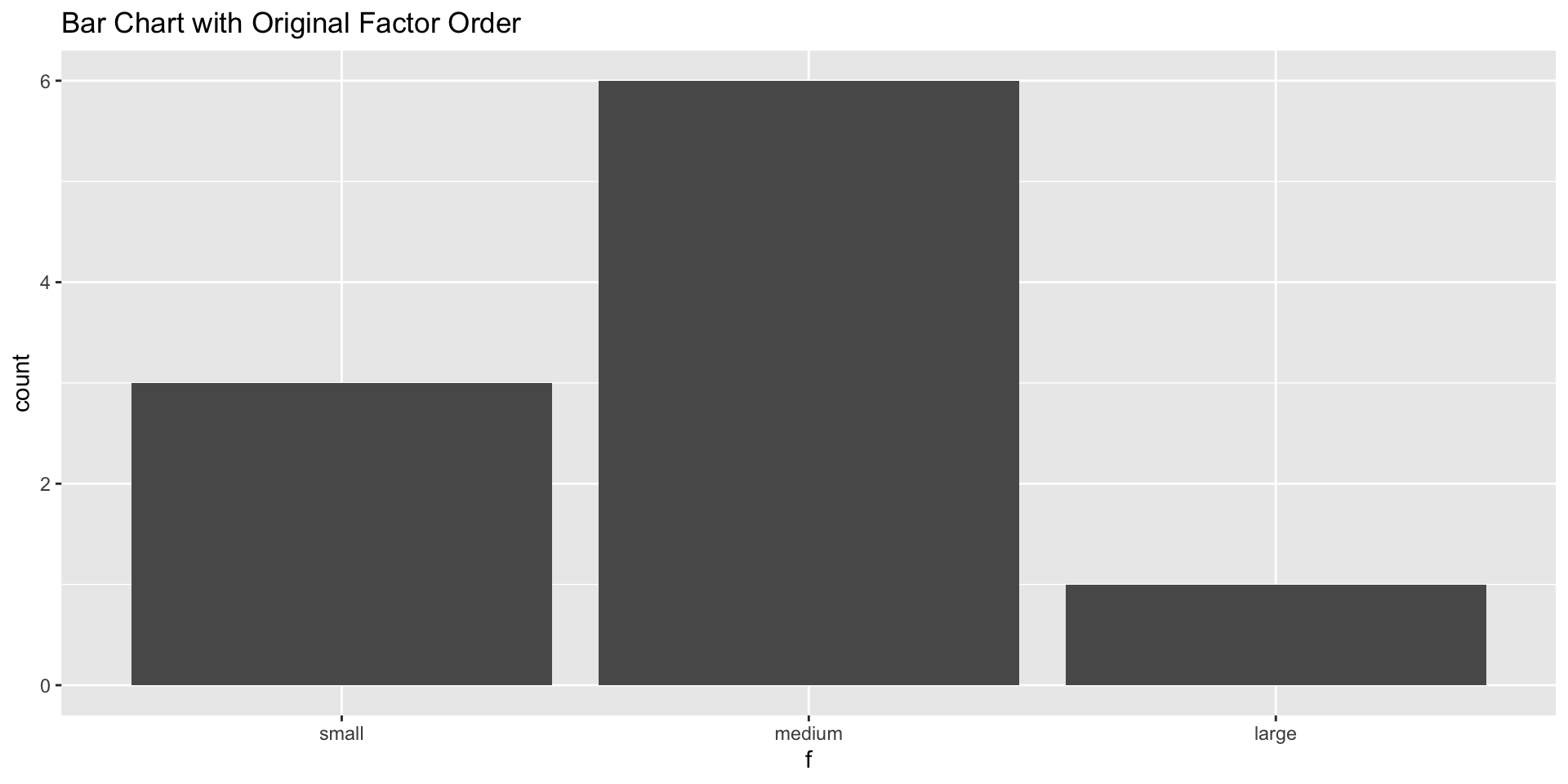
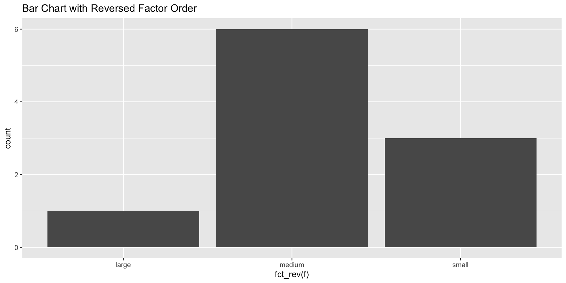
fct_rev use case: flip bar chart

Use case: Flip bar chart from top-to-bottom to bottom-to-top

ggplot(data.frame(f), aes(x = f)) + 
  geom_bar() +
  labs(title = "Bar Chart with Original Factor Order")

ggplot(data.frame(f), aes(x = fct_rev(f))) +
  geom_bar() +
  labs(title = "Bar Chart with Reversed Factor Order")

Reorder: by appearance

fct_inorder(): Order by first appearance

f <- factor(c("b", "b", "a", "c", "c", "c"))
f

[1] b b a c c c
Levels: a b c

Reorder by first appearance

fct_inorder(f)

[1] b b a c c c
Levels: b a c

Equivalent to creating with as_factor()

f <- as_factor(c("b", "b", "a", "c", "c", "c"))
f

[1] b b a c c c
Levels: b a c

Reorder: by frequency

fct_infreq(): Reorder from most to least common

f <- factor(c("b", "b", "a", "c", "c", "c"))
f

[1] b b a c c c
Levels: a b c

Reorder by frequency, most common first

fct_infreq(f)

[1] b b a c c c
Levels: c b a

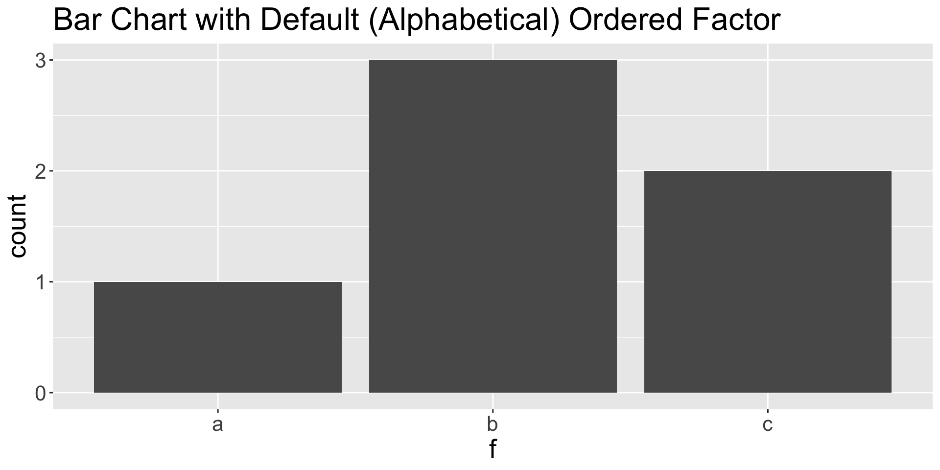
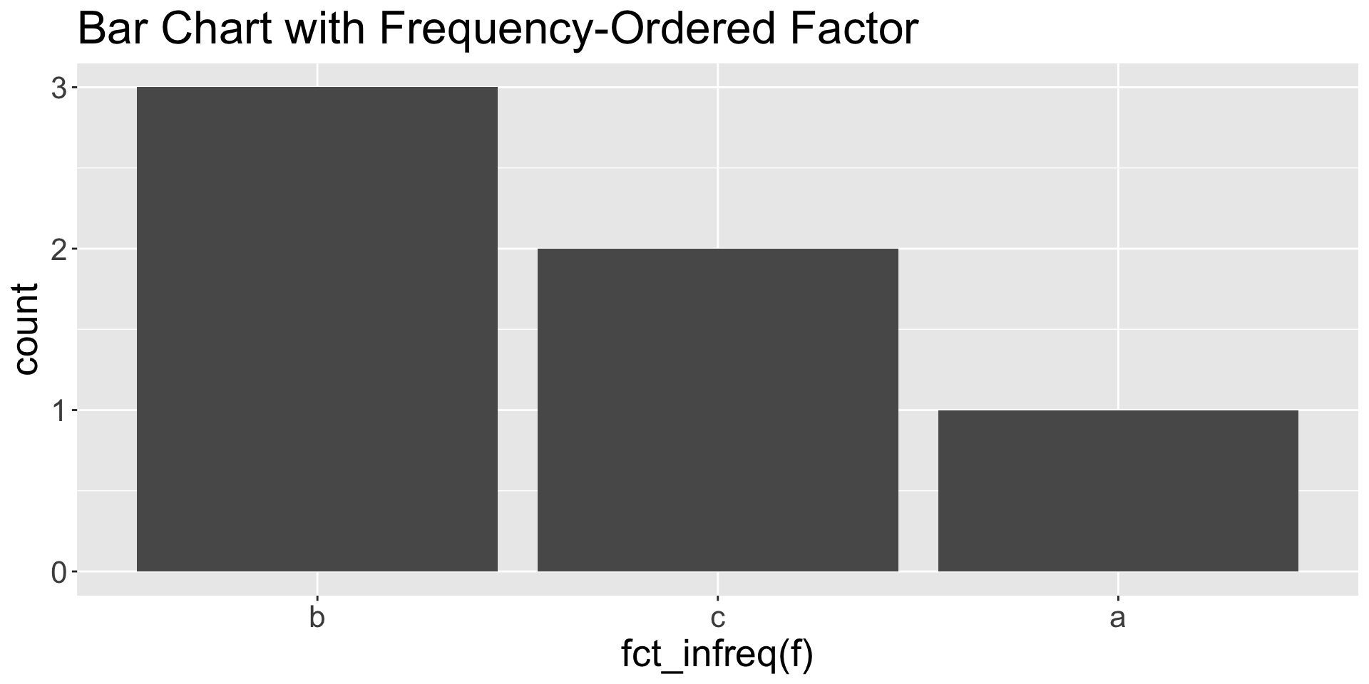
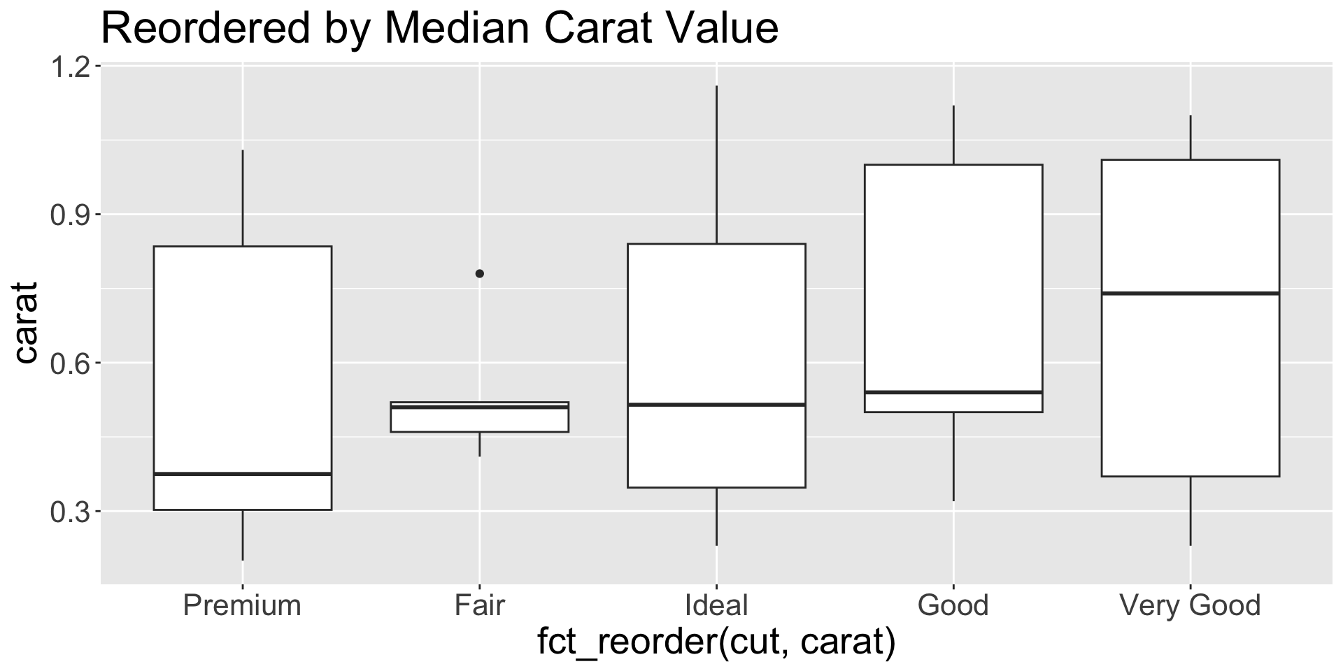
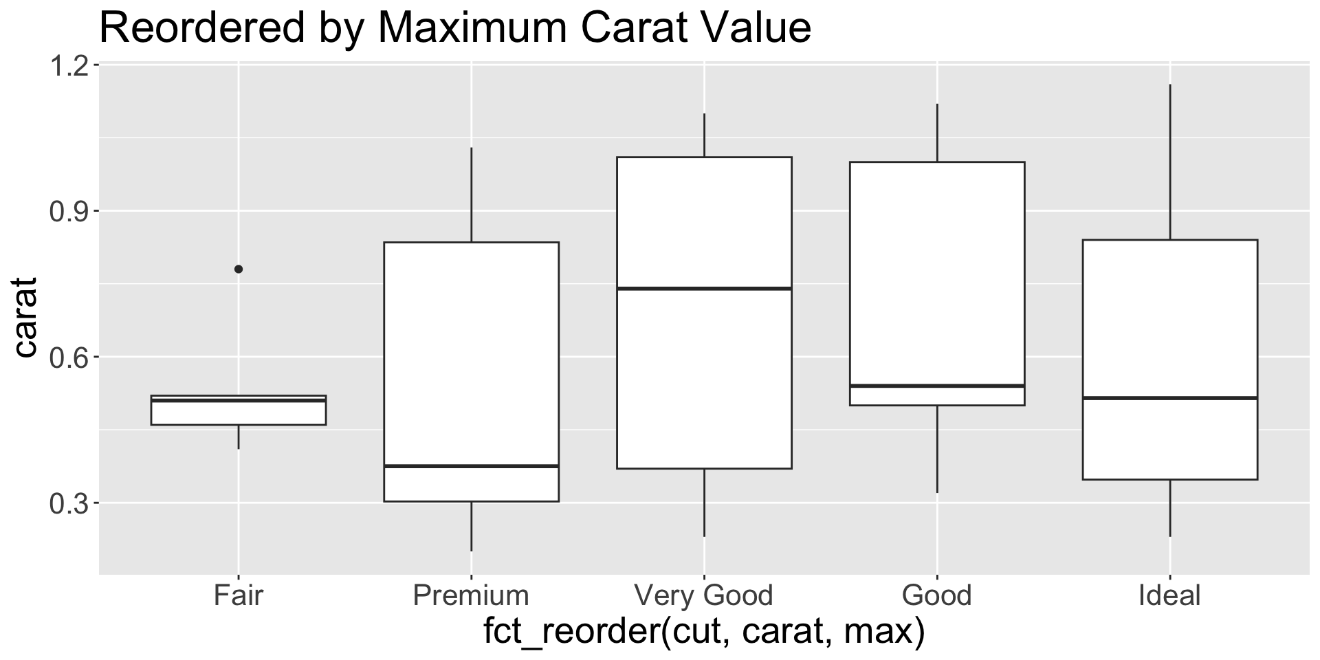
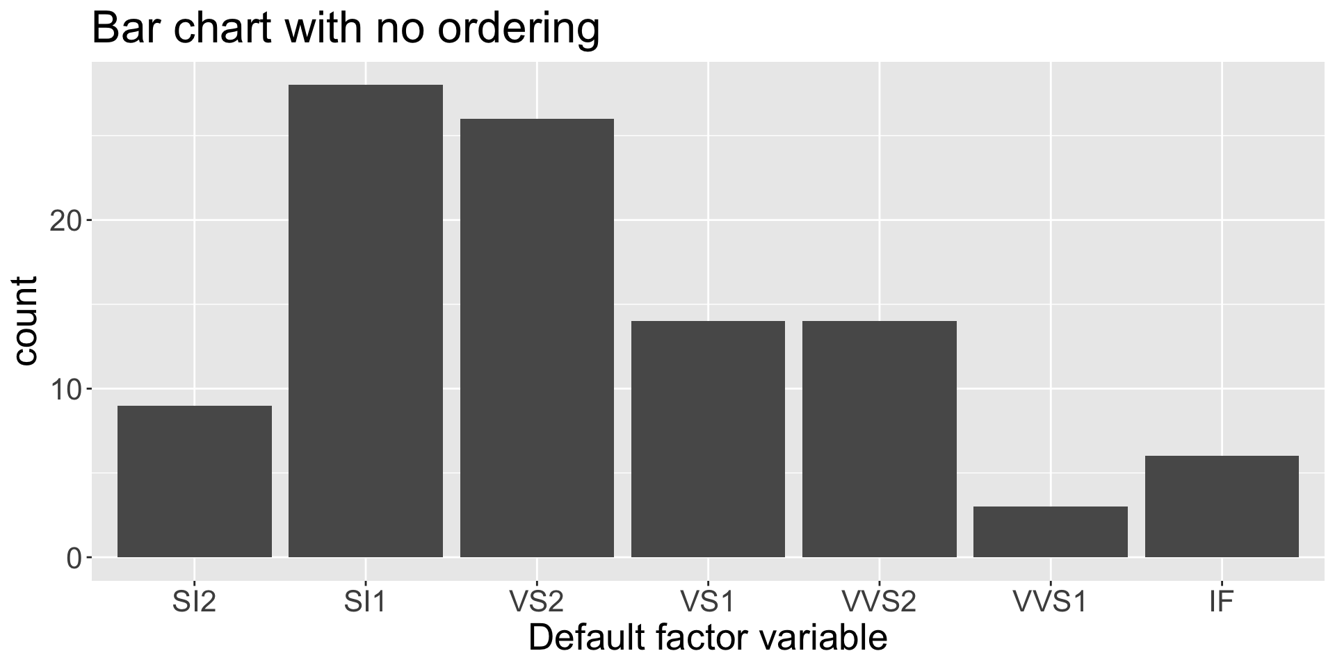
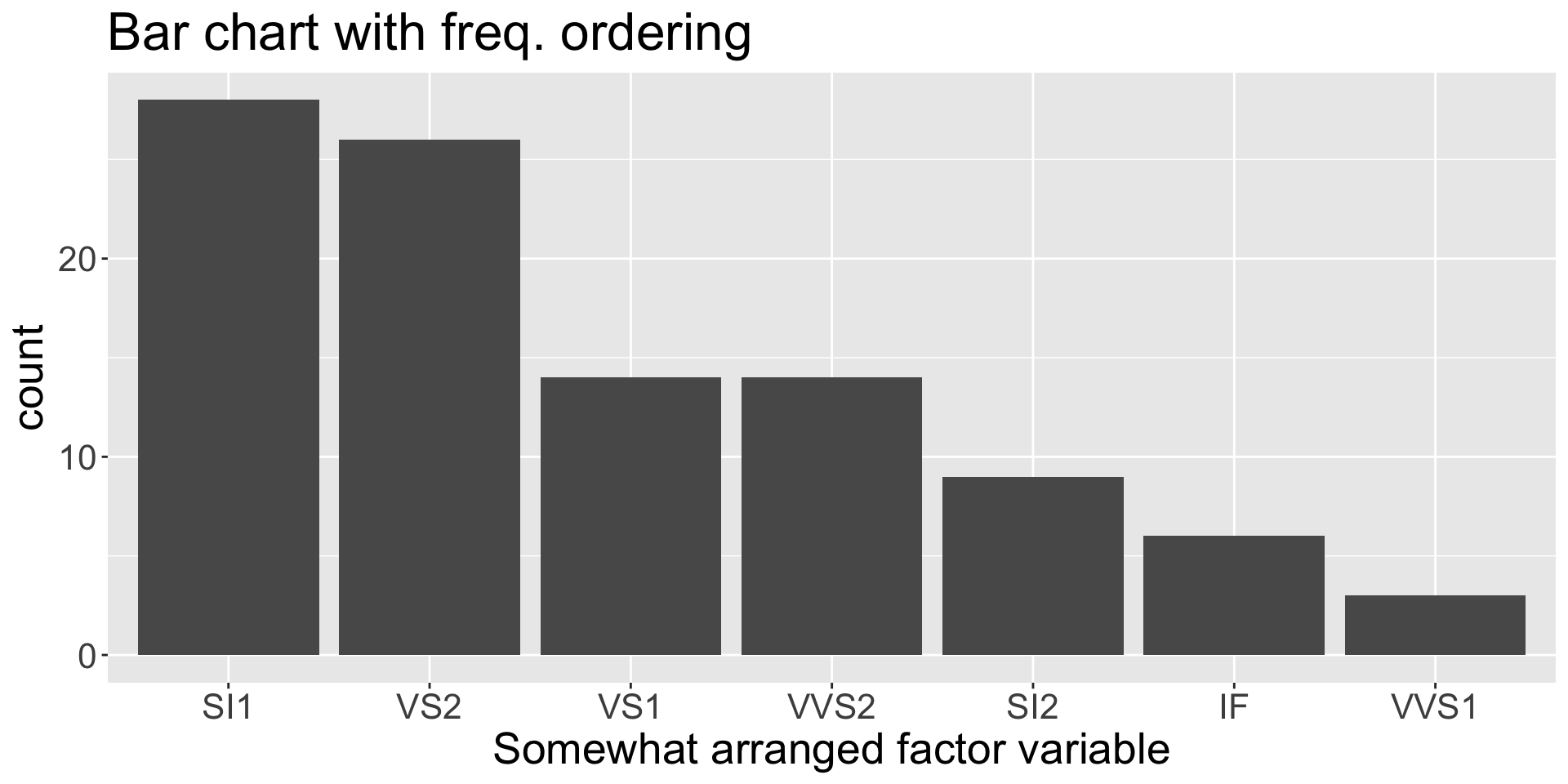
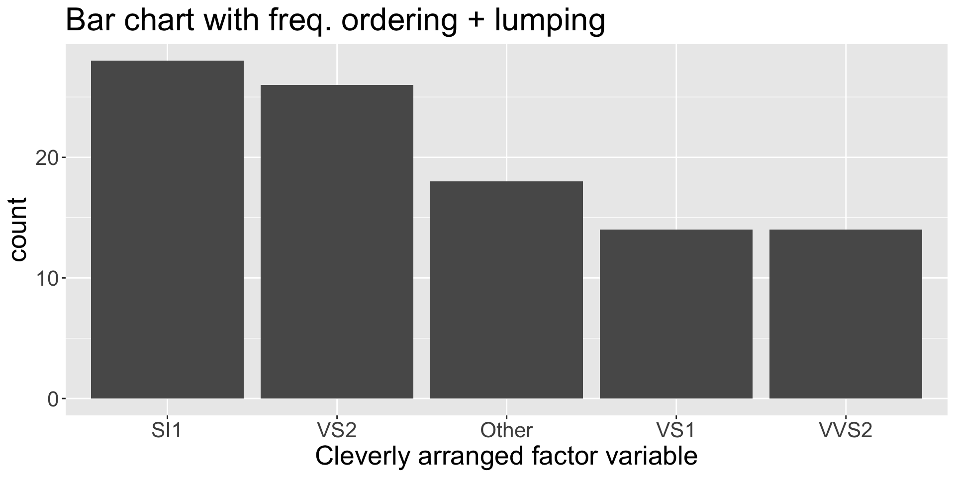
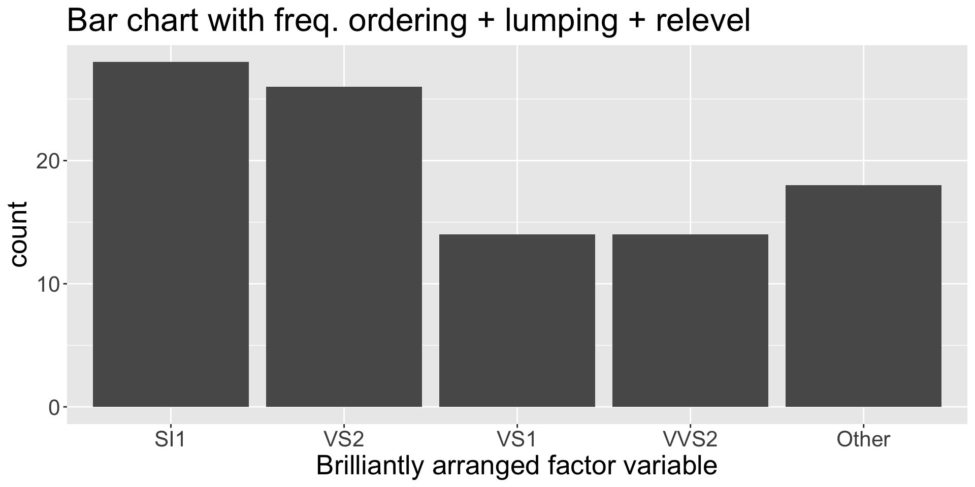
fct_infreq use case: interpretable bar charts

f <- factor(c("b", "b", "b", "a", "c", "c"))

ggplot(data.frame(f), aes(x = f)) +
    geom_bar() +
    labs(title =
        "Bar Chart with Default (Alphabetical) Ordered Factor") +
    theme(text = element_text(size = 20))

ggplot(data.frame(f), aes(x = fct_infreq(f))) +
    geom_bar() +
    labs(title =
        "Bar Chart with Frequency-Ordered Factor") +
    theme(text = element_text(size = 20))

Probably the most common use case for fct_infreq() is to create bar charts with bars ordered by frequency (most common first). This is often more informative than the default alphabetical ordering.

Reorder: by another variable (summary)

fct_reorder(f, x, fun): Order factor by summary of another variable

Default: sort by level median

ggplot(diamonds_100, aes(
    x = fct_reorder(cut, carat), y = carat)) +
    geom_boxplot() +
    labs(title = "Reordered by Median Carat Value") +
    theme(text = element_text(size = 20))

Or sort by any other summary function, e.g., max

ggplot(diamonds_100, aes(
    x = fct_reorder(cut, carat, max), y = carat)) +
    geom_boxplot() +
    labs(title = "Reordered by Maximum Carat Value") +
    theme(text = element_text(size = 20))

Reorder: by another variable (relationship)

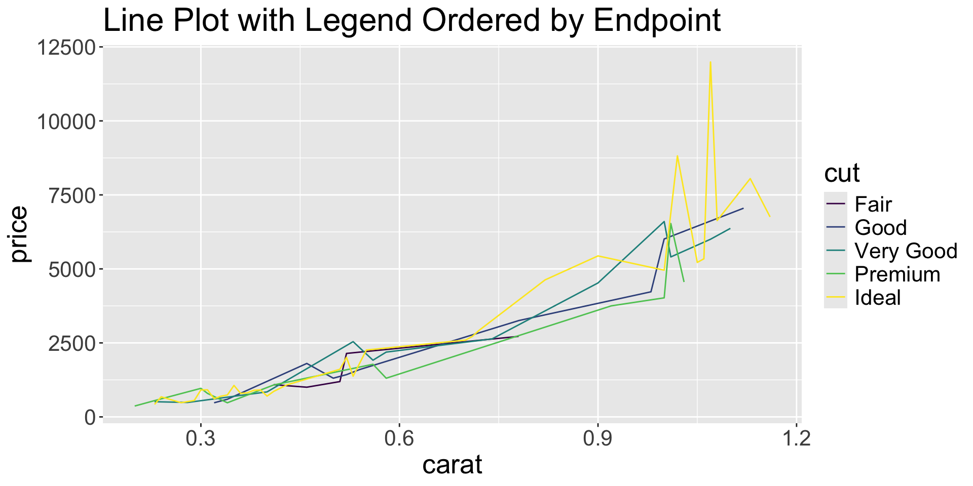
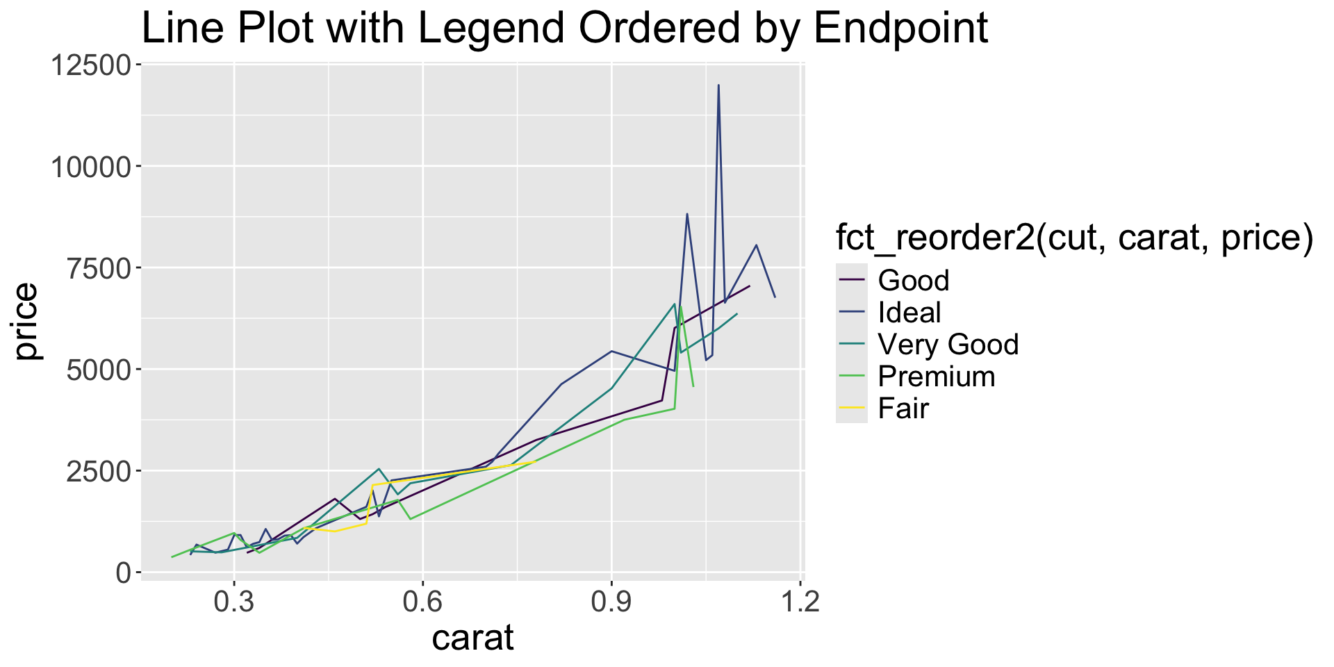
fct_reorder2(f, x, y): Order by relationship with two variables (great for line plots)

Line plot without reorder

diamonds_100 |> 
    ggplot(aes(x = carat, y = price, 
        color = cut)) +
    geom_line(stat = "summary", fun = mean) +
    labs(title = "Line Plot with Legend Ordered by Endpoint") +
    theme(text = element_text(size = 20))

Compare last values of y for each level of f across x

diamonds_100 |> 
    ggplot(aes(x = carat, y = price, 
        color = fct_reorder2(cut, carat, price))) +
    geom_line(stat = "summary", fun = mean) +
    labs(title = "Line Plot with Legend Ordered by Endpoint") +
    theme(text = element_text(size = 20))

Notice that if you use a forcats variable like fct_reorder on a non-factor variable, it will convert it to a factor with the new order. This is a common way to reorder factors on the fly for plotting without needing to create a new variable in your dataset.

Reassign Factor Levels

Reassign: rename levels

fct_recode(): Manually rename specific levels new_name = "old_name"

Create factor with messy level names

f <- factor(c("Low ", "Medium", "High", "Medium ", "Low", "high", "Hihg"))
f

[1] Low     Medium  High    Medium  Low     high    Hihg   
Levels: high High Hihg Low Low  Medium Medium 

Clean up names. Map multiple old levels to same new or existing level individually.

f_clean <- fct_recode(f,
                      Low = "Low ",
                      Medium = "Medium ",
                      High = "high",
                      High = "Hihg")

f_clean

[1] Low    Medium High   Medium Low    High   High  
Levels: High Low Medium

You can create new codes and they don’t have to be strings

Reassign: collapse levels manually

fct_collapse(): Combine multiple levels into one new_name = c("old1", "old2")

f <- factor(c("A", "A", "B", "B", "B", "C", "C", "C", "C", "D", "E", "F", "G", "G", "G", "G", "G"))

f_collapsed <- fct_collapse(
    f,
    Group1 = c("A", "B"),
    Group2 = c("C", "D"),
    Group3 = "E")

f_collapsed

 [1] Group1 Group1 Group1 Group1 Group1 Group2 Group2 Group2 Group2 Group2
[11] Group3 F      G      G      G      G      G     
Levels: Group1 Group2 Group3 F G

Reassign: lump levels manually

fct_other(): Lump (non/)specified levels into “Other”

f <- factor(c("A", "A", "B", "B", "B", "C", "C", "C", "C", "D", "E", "F", "G", "G", "G", "G", "G"))

fct_other(f, keep = c("A", "B", "C"))

 [1] A     A     B     B     B     C     C     C     C     Other Other Other
[13] Other Other Other Other Other
Levels: A B C Other

fct_other(f, drop = c("A", "B", "C"))

 [1] Other Other Other Other Other Other Other Other Other D     E     F    
[13] G     G     G     G     G    
Levels: D E F G Other

“Lumping” is not the same as “dropping” despite the argument being “drop.” It creates an “other” level, remaps levels to “other”, then drops unused levels.

Reassign: lump levels automatically

fct_lump_*() family: Keep levels by condition, lump rest into “Other”

f <- factor(c("A", "A", "B", "B", "B", "C", "C", "C", "C", "D", "E", "F", "G", "G", "G", "G", "G"))

fct_lump_n(): keep most frequent N

fct_lump_n(f, n = 3)

 [1] Other Other B     B     B     C     C     C     C     Other Other Other
[13] G     G     G     G     G    
Levels: B C G Other

fct_lump_prop(): keep levels above percent frequency

fct_lump_prop(f, prop = 0.2)

 [1] Other Other Other Other Other C     C     C     C     Other Other Other
[13] G     G     G     G     G    
Levels: C G Other

fct_lump_min(): keep levels with at least N observations

fct_lump_min(f, min = 4)

 [1] Other Other Other Other Other C     C     C     C     Other Other Other
[13] G     G     G     G     G    
Levels: C G Other

Collapsing levels: Use fct_collapse() to combine multiple levels into single level. Show fct_lump() to automatically lump least common levels into “Other”. Demonstrate fct_lump_n(), fct_lump_prop(), fct_lump_min() for different lumping strategies.

Add/Drop Levels

Add/Drop: add and remove levels

fct_expand(): Add new levels without observations

f_abc <- factor(c("A", "B", "C"))
f_abc

[1] A B C
Levels: A B C

fct_expand(f, "D", "E")

 [1] A A B B B C C C C D E F G G G G G
Levels: A B C D E F G

fct_drop(): Remove levels with no observations

f_abcde <- factor(c("A", "B", "C"), 
    levels = c("A", "B", "C", "D", "E"))
f_abcde

[1] A B C
Levels: A B C D E

fct_drop(f_abcde)

[1] A B C
Levels: A B C

In combination

# add unused levels
fct_expand(f_abc, "D", "E") |> 
    # then drop them
    fct_drop()

[1] A B C
Levels: A B C

fct_drop use case: tibble filter

# Create a tibble with a factor variable
t <- tibble(
    f = factor(c("A", "B", "C", "D", "E")),
    i = c(1:5)
)

t

# A tibble: 5 × 2
  f         i
  <fct> <int>
1 A         1
2 B         2
3 C         3
4 D         4
5 E         5

t$f

[1] A B C D E
Levels: A B C D E

t_subset <- filter(t, i <= 3)
t_subset$f

[1] A B C
Levels: A B C D E

fct_drop(t_subset$f)

[1] A B C
Levels: A B C

Dropping unused levels: Compare droplevels() with fct_drop() to remove levels with no observations. Commonly used after filtering data.

Add/Drop: handle missing values

fct_na_value_to_level(): Convert between NA values and NA levels

f <- factor(c("A", "B", NA, "A", "C", NA, "B"))
f

[1] A    B    <NA> A    C    <NA> B   
Levels: A B C

Create explicit NA level

fct_na_value_to_level(f)

[1] A    B    <NA> A    C    <NA> B   
Levels: A B C <NA>

Convert NAs to named level

fct_na_value_to_level(f, level = "(Missing)")

[1] A         B         (Missing) A         C         (Missing) B        
Levels: A B C (Missing)

WHY? - Make missingness visible in plots - Include NAs in counts and summaries

fct_explicit_na() is deprecated, but you’ll still see it and it still works. The new name fct_na_value_to_level() is more descriptive of what the function actually does, which is to convert NA to explicit “(Something)” level.

See Also

forcats functions we didn’t talk about:

1. Create: n/a – just as_factor()
2. Inspect:
   1. fct_match(f, lvls): check for levels in f
3. Combine:
   1. fct_cross(f1, f2): Create interaction factor
4. Reorder
   1. fct_inseq(): Order by natural sequence
   2. fct_shift(): Shift levels L or R, wrapping around
   3. fct_shuffle(): Randomly permute levels
5. Modify
   1. fct_lump_lowfreq(): Lump low-frequency levels
   2. fct_relabel(): Rename levels with function
   3. fct_anon(): Anonymize to random integers

Practical Applications

Data cleaning workflow

String cleaning → Factor creation

Common workflow:

1. Trim whitespace
2. Standardize case
3. Fix inconsistencies
4. Convert to factor

Messy categorical (string) data with inconsistent entries

# Create messy data
messy <- c(" Low", "medium ", "HIGH", "medium", " low", "high", NA, "Hihg")

Pipeline wth str and factor creation in one step

messy |> 
    str_trim() |> 
    str_to_lower() |> 
    str_replace("hihg", "high") |> 
    factor(levels = c("low", "medium", "high"), 
        ordered = TRUE) |> 
    fct_na_value_to_level("no response")

[1] low         medium      high        medium      low         high       
[7] no response high       
Levels: low < medium < high < no response

Data cleaning workflows: Demonstrate pipeline combining string cleaning (trimming, case conversion) with factor creation. Show fixing inconsistent categorical entries.

Visualization preparation

Make better plots with factor control

• Reorder for sorted bars (fct_infreq, fct_reorder)
• Collapse rare categories (fct_lump_*)
• Control legend order

Visualization preparation

Create a simple bar chart

diamonds_100 |> 
    ggplot(aes(x = clarity)) +
    geom_bar() +
    labs(title = "Bar chart with no ordering",
        x = "Default factor variable")

Visualization preparation

Reorder factor by decreasing frequency

diamonds_100 |> 
ggplot(aes(x = 
        fct_infreq(clarity))) +
geom_bar() +
labs(title = "Bar chart with freq. ordering",
    x = "Somewhat arranged factor variable")

Visualization preparation

Lump rare categories for cleaner visualization

diamonds_100 |> 
ggplot(aes(x = 
        fct_lump_n(clarity, n = 4) |> 
        fct_infreq())) +
geom_bar() +
labs(title = "Bar chart with freq. 
    ordering + lumping",
    x = "Cleverly arranged factor variable")

Visualization preparation

Move “other” level to the end

diamonds_100 |> 
ggplot(aes(x = 
        fct_lump_n(clarity, n = 4) |> 
        fct_infreq() |> 
        fct_relevel("Other", 
            after = Inf))) +
geom_bar() +
labs(title = "Bar chart with freq. 
    ordering + lumping + relevel",
    x = "Brilliantly arranged factor variable")

Preparing data for visualization: Show reordering factors for sorted bar charts and line plots. Demonstrate collapsing rare categories for cleaner plots. Illustrate controlling legend order.

Modeling categorical data

Factor order matters in models! The first level is the reference category. Example: using mtcars data, predict mpg using cyl (number of cylinders) as a factor variable.

Fit regression model with cyl as factor

summary(
    lm(mpg ~ factor(cyl), data = mtcars)
)

Call:
lm(formula = mpg ~ factor(cyl), data = mtcars)

Residuals:
    Min      1Q  Median      3Q     Max 
-5.2636 -1.8357  0.0286  1.3893  7.2364 

Coefficients:
             Estimate Std. Error t value Pr(>|t|)    
(Intercept)   26.6636     0.9718  27.437  < 2e-16 ***
factor(cyl)6  -6.9208     1.5583  -4.441 0.000119 ***
factor(cyl)8 -11.5636     1.2986  -8.905 8.57e-10 ***
---
Signif. codes:  0 '***' 0.001 '**' 0.01 '*' 0.05 '.' 0.1 ' ' 1

Residual standard error: 3.223 on 29 degrees of freedom
Multiple R-squared:  0.7325,    Adjusted R-squared:  0.714 
F-statistic:  39.7 on 2 and 29 DF,  p-value: 4.979e-09

Use fct_rev() to change reference level

summary(
    lm(mpg ~ fct_rev(factor(cyl)), data = mtcars)
)

Call:
lm(formula = mpg ~ fct_rev(factor(cyl)), data = mtcars)

Residuals:
    Min      1Q  Median      3Q     Max 
-5.2636 -1.8357  0.0286  1.3893  7.2364 

Coefficients:
                      Estimate Std. Error t value Pr(>|t|)    
(Intercept)            15.1000     0.8614  17.529  < 2e-16 ***
fct_rev(factor(cyl))6   4.6429     1.4920   3.112  0.00415 ** 
fct_rev(factor(cyl))4  11.5636     1.2986   8.905 8.57e-10 ***
---
Signif. codes:  0 '***' 0.001 '**' 0.01 '*' 0.05 '.' 0.1 ' ' 1

Residual standard error: 3.223 on 29 degrees of freedom
Multiple R-squared:  0.7325,    Adjusted R-squared:  0.714 
F-statistic:  39.7 on 2 and 29 DF,  p-value: 4.979e-09

The first level is the “dummy” or reference category. Output is only interpretable in relation to that first level.