vector_structure <- c(25, 30)
vector_structure
[1] 25 30| name | abbr. | definition | examples | notes |
|---|---|---|---|---|
| logical | lgl | booleans, binary yes/no | TRUE FALSE |
|
| integer | int | self-explanatory | 1L 20L |
needs L after number to force integer type |
| double | dbl | non-integer numbers | 1 20.0 |
default numeric storage type |
| complex | cplx | complex numbers like imaginaries | i |
ignore for now |
| character | chr | strings, located within quotation marks | "a" "marky mark" |
typeof() / class()
typeof() will differentiate between integer and double. class() will return numeric for bothas.logical(), as.character(), as.double(), as.numeric()
as.logical("Mary") would be impossible| structure | dimensions | mixed elements? | notes |
|---|---|---|---|
| vector | 1d | no | all elements must be same type |
| matrix | 2d | no | all elements must be same type |
| dataframe | 2d | yes (column) | each column is a vector |
| list | flexible | yes | can contain all element types |
ifelse() (vectorized) vs. if () ... else if () (non-vectorized)length()
class()
typeof() isn’t as helpful with data structuresas.array(), as.data.frame(), as.matrix(), as.list()
go here for vector subsetting
vector_structure <- c(25, 30)
vector_structure[1] 25 30c(1)c(25, 30) + c(25, 30) # same length, no warning[1] 50 60c(25, 30) + c(25, 30, 35, 40) # different lengths but factorable lengths, no warning[1] 50 60 60 70c(25, 30) + c(25, 30, 35) # different lengths, NOT factorable lengths, warningWarning in c(25, 30) + c(25, 30, 35): longer object length is not a multiple of
shorter object length[1] 50 60 60go here for matrix subsetting
matrix_structure <- matrix(25:30, nrow = 2, ncol = 3)
matrix_structure
[,1] [,2] [,3]
[1,] 25 27 29
[2,] 26 28 30go here for dataframe subsetting
dataframe_structure <- data.frame(name = c("A", "B"), age = c(25L, 30L), bday = c(1.1, 2.2), vector_structure)
dataframe_structure
name age bday vector_structure
1 A 25 1.1 25
2 B 30 2.2 30go here for list subsetting
list_structure <- list(name = c("A", "B"), age = c(25L, 30L, 35L), bday = c(1.1, 2.2), age_mix = c(25L, 30.25), dataframe_structure, vector_structure)
list_structure$name
[1] "A" "B"
$age
[1] 25 30 35
$bday
[1] 1.1 2.2
$age_mix
[1] 25.00 30.25
[[5]]
  name age bday vector_structure
1    A  25  1.1               25
2    B  30  2.2               30
[[6]]
[1] 25 30[single brackets]vector_structure[1] # 1st element[1] 25vector_structure[c(1, 2)] # 1st and 2nd element[1] 25 30vector_structure[-1] # all elements except the 1st[1] 30vector_structure[vector_structure < 30] # all elements smaller than 30[1] 25[row, column] argumentation with single bracketsmatrix_structure[1, 2] # element at row 1, column 2[1] 27matrix_structure[2, ] # entire row 2[1] 26 28 30matrix_structure[ , 2] # entire column 2[1] 27 28matrix_structure[1:2, 3] # submatrix of rows 1-2 and column 3[1] 29 30matrix_structure[ , c(1, 3)] # columns 1 and 3 [,1] [,2]
[1,] 25 29
[2,] 26 30dataframe_structure[1, ] # dataframe of 1st row with all columns name age bday vector_structure
1 A 25 1.1 25dataframe_structure[ , 2] # vector of 2nd column with all rows[1] 25 30dataframe_structure["name"] # dataframe of "name" column name
1 A
2 Bdataframe_structure[ , "name"] # vector of "name" column[1] "A" "B"dataframe_structure$name # vector of "name" column[1] "A" "B"dataframe_structure$name[2] # vector of value at 2nd row, "name" column[1] "B"dataframe_structure[["name"]] # vector of "name" column[1] "A" "B"dataframe_structure[1, 2] # vector of value at 1st row, 2nd column[1] 25dataframe_structure[1:2, "name"] # vector of rows 1 - 2, "name" column[1] "A" "B"dataframe_structure[[1]] # dataframe of 1st column[1] "A" "B"[single brackets] to get a sublist
[[double brackets]] or $dollarsign
list_structure[1] # list of 1st element's contents$name
[1] "A" "B"list_structure[[1]] # vector of 1st element's contents[1] "A" "B"list_structure[[1]][2] # vector of 1st element's 2nd value[1] "B"list_structure["name"] # list of element "name"'s contents$name
[1] "A" "B"list_structure$name # vector of element "name"'s contents[1] "A" "B"list_structure$name[2] # vector of element "name"'s 2nd value[1] "B"list_structure[["name"]] # vector of element "name"'s contents[1] "A" "B"list_structure[["name"]][2] # vector of element "name"'s 2nd value[1] "B"# arithmetic operators
x + y
x - y
x * y
x / y
x ^ y
x %% y # modulus; returns the remainder of x/y
x %/% y # integer division; returns the whole number result of x/y
# assignment operators
x <- 2 # used for assigning values to objects
mean(x = c(1, 2)) # used to specify what arguments should evaluate to within functions
# comparison operators
x == x # x equals x
x != y # x does NOT equal y
x > y # x is greater than y
x < y # x is less than y
x >= y # x is greater than or equal to y
x <= y # x is less than or equal to y
# logical operators (combine comparison statements)
logic_x & logic_y # vectorized AND; logic_x AND logic_y are true
logic_x && logic_y # non-vectorized AND; logic_x AND logic_y are true. not used very often
logic_x ! logic_y # NOT; logic_x NOT logic_y. can be combined with other operators
logic_x | logic_y # vectorized OR; logic_x OR logic_y are true
logic_x || logic_y # non-vectorized OR; logic_x OR logic_y are true. not used very often
# misc operators
1:2 # 1 through 2
element_x %in% vector_y # element_x is in vector_y
matrix_x %*% matrix_y # matrix multiplication
dependent_x ~ independent_y # separates dependent and independent variables in formulas that specify relationships between variableshead()
head(dataset)tail()
tail(dataset)paste(), paste0()apply()apply(dataset, vector_of_operating_dimension, function)
vector_of_operating_dimension, using 1 will apply the function over rows, 2 over columns, and c(1, 2) over rows and columnslapply(), sapply(), vapply()lapply() returns a list the same length as the input datasetsapply() returns a vector or matrix
lapply() with more possible arguments and customizationvapply() is similar to sapply() but requires an argument that specifies how the return will be formattedif ()else ()while ()
when() condition eventually endswhile() conditionals can be written as for() loops, but not all for() loops can be written as while() conditionalsfor () loops in r: over elements or over index positionsfor (element in vector_structure)) {
element == literal_value_of_element_in_the_vector
}for (i in seq_along:vector_structure)) {
vector_structure[i] == whatever_value_is_in_position_number_i_in_vector_structure
i == number_of_loops
}
# note: the `i` here can be named anything you want
# using `i` for index positions is most common
# personally it reminds me i'm looking at positions, not elementsstop()
return()
{{ }} only gets used to refer to an argument when incorporating tidy evaluations into a user-defined function
see here for an exhaustive list of functions in dplyr
select()select(dataset, arguments_for_selecting_columns_here)select(dataset, new_name = old_name)select(dataset, column_3, column_1, column_2)starts_with("prefix"), ends_with("suffix"), contains("text"), matches("regex")where(function())
function() evaluates to TRUEeverything()
vars = c() where c() is a vector of variable namesvars = is left empty, takes all variables from the current context/piperename()rename(dataset, new_name = old_name)relocate()relocate(dataset, column_3, .before = column_2, .after = column_1)mutate()mutate(dataset, new_column_1 = ..., new_column_2 = ...)glimpse()glimpse(dataset)across()filter()filter(dataset, filter_variable)arrange()arrange(dataset, column_1, column_2)arrange(dataset, desc(column_1))distinct()distinct(dataset, .keep_all = FALSE)
.keep_all = TRUE, all variables in the dataset are retainedsummarize()mean(), sd(), min(), max(), etc.summarize(dataset, col_name = operation())rowwise()group_by()summarize() or count()group_by(dataset, grouping_variable)count()count(dataset, grouping_variable)case_when()if_else()recode_values() and replace_values()pivot_longer()
pivot_wider()
separate()
unite()
ggplot(dataset, mapping = aes())mapping = aes()) are inherited by the geoms set afterwardssee here for more geom types
geom_point()stat = "identity"geom_hline(), geom_vline(), geom_abline()linetype can range from 0 to 6 (preset line types)
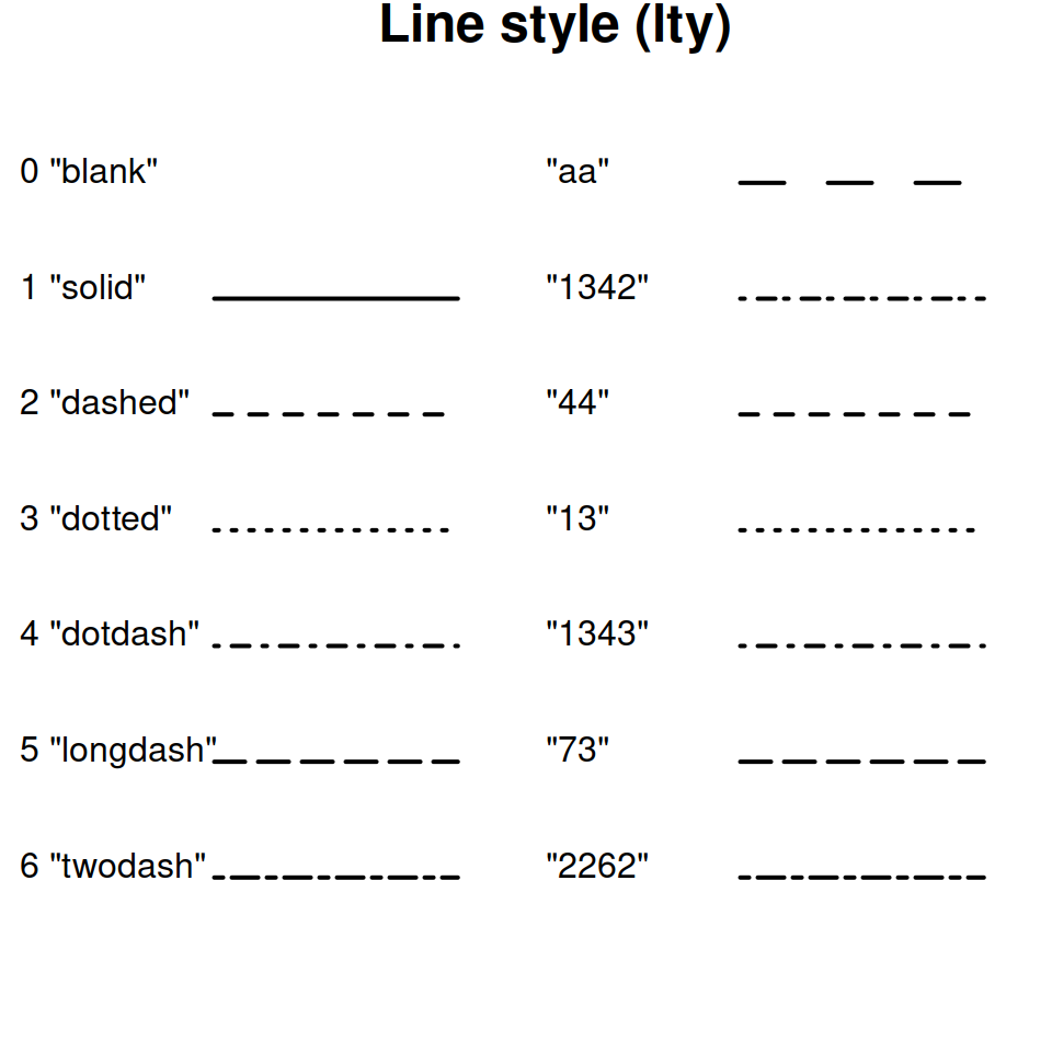
linewidth is set in mmgeom_smooth()method = which allows you to specify what type of function to use
method = "loess" (local polynomial regression fitting) when there are over 1,000 observationsmethod = "lm" (linear model) when there are under 1,000 observationsformula = which allows you to specify the specific formula using x and y
formula = NULLgeom_bar()position = "stack"stat = "count"x is categorical, you can go from a stacked bar chart to a grouped/clustered bar chart using position = "dodge"geom_histogram()geom_boxplot()geom_area()geom_text(), geom_label()geom_text() only creates text
check_overlap = to see if it’s overlapping other text
TRUE will make sure the text does not overlap with other text, FALSE will let it do sogeom_label() will create text that has a rectangle behind it, making it easier to readlabel = to tell it what to sayx = is needed for mapping any ggplot
y = is sometimes required; will default to "stat = identity" in specific geoms that require a y argument and "stat = count" when optional
"identity" means it will use y as the y-axis plotting variable"count" means it will try to count the instances of x and use that as the y-axis plotting variablefill is background/inside color
color is outlinealpha is transparency (100 = opaque, 0 = completely transparent)size is self explanatoryshape is the shape of the point
NA for nothing 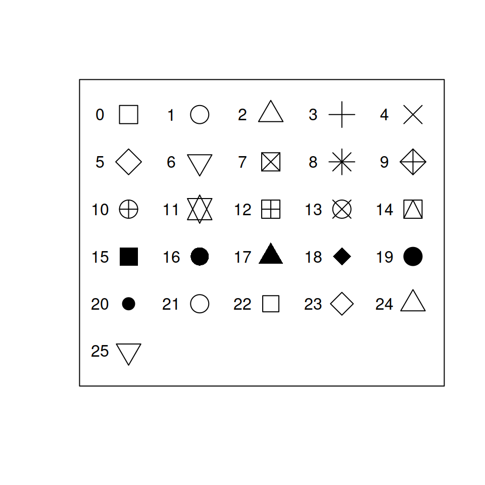
fill argumentcolor argumentif_else()labs
x =, y =, and title =subtitle = "Your text here" will create text below the titlecaption = "Your text here" will create text displayed to the bottom-right of the plot
tag = "Your text here" will create text displayed to the top-left of the plot
color = "Groups" to title the color legend “Groups” instead of the name of the raw variable= NULL and get rid of it completely
= "")lims()
(x = c(lower_x_limit, upper_x_limit), y = c(lower_y_limit, upper_y_limit)scale_x_discrete()/scale_y_discrete
labels = c("Label 1", "Label 2") controls the text of the labels for the axis ticksscale_x_continuous()/scale_y_continuous
n.breaks = controls the number of major ticks along the axisbreaks = c() controls the exact ticks that will show uplabels = controls the format of the tick labels
scales::percentscales::label_dollarfacet_wrap()facets = "grouping_variable"
group_by()nrow = insert_number_of_rows_herencol = insert_number_of_columns_herescales =
"fixed", the minimum and maximum value for the x axes and y axes will be the same across all plots
"free_x" or "free_y", the specified axis will change according to the values of each plot"free", both the x and y axes will change according to the values of the plotguide() layerguide_legend()guide_axis()
angle =, lets you angle the textguide = guide_axis()str_view()
str_detect()
str_count()
str_extract(), str_extract_all()
str_replace(), str_replace_all()
str_split()
map()
fct_relevel()
fct_infreq()
fct_reorder()
make_datetime()
ymd(), mdy(), dmy()
year(), month(), day(), wday()