In this chapter we will go into a bit more depth on some of what we covered in ?sec-r-language-basics, and introduce some more complicated programming concepts you’re likely to need as a social sciences researcher.
7.2 Essential concepts
7.2.1 Object assignment
In R we create variables by assigning a value to a name with the assignment operator <-. Technically you can use = to assign a value to a variable, but you really shouldn’t; <-is the preferred assignment operator in R.
7.2.2 Indexing and subsetting with [ ] & $
use : to create a vector of integers beginning with one number and ending with another
1:5 is equivalent to c(1, 2, 3, 4, 5)
use [ and ] to select elements of a vector, list, or data frame by position or name
c(1, 10, 3, 1000, 2)[4] returns the fourth element of the vector, 1000
use , to separate row and column indices when selecting from a data frame or matrix
mtcars[1, ] returns the first row of the mtcars data frame
mtcars[, 1] returns the first column of the mtcars data frame
mtcars[1, 1] returns the value in the first row and first column of the mtcars data frame
use [[ and ]] to select a single list element by position or name
How are [ and [[ different? [ always returns an object of the same type as the original object, while [[ returns a single element of the object. This starts to matter when you’re working with complex data structures that store multiple data types, like lists, data frames, and model output.
# Create a list with two elements: a numeric vector and a character vectormixed_list <-list(a =1:5, b = letters[1:5])
We introduced functions in ?sec-function-basics, and you’ll have seen them used throughout course materials so far. There’s just no sensible way to talk about anything in R without implicitly using some functions, so hopefully by now you’ve picked up on the gist of how they work. You can honestly get pretty just using functions without understanding them, but obviously you can get a lot farther if you do, so let’s talk about them a bit more.
Here’s a thing that is definitely totally hypothetical and has never happened:
I ignore my work and start playing my favorite video game.
“Ignoring” and “playing” are functions, and “my work” and “my favorite video game” are the objects those functions are acting on.
7.3.1 Function arguments and return values
When you want to do the action (or more analogous to R, when you want to tell someone to do the action), you’ll often want to add some more information to specify what exactly you want to do the action to or how to do it.
7.3.2 Writing functions
7.3.2.1 Anonymous functions
An anonymous function is a function that is defined without being assigned to a name. This is useful for short, one-off functions that you don’t need to reuse elsewhere in your code. You’re most likely to need anonymous functions when you’re using functions that take other functions as arguments, like sapply()1. For example:
# Use an anonymous function to square each element of a vectorsquare_them_all <-sapply(1:5, function(x) x^2)print(square_them_all) # returns: [1] 1 4 9 16 25
The sapply() function takes a function as an argument and applies it to each element of a vector or list (in this case, the series of numbers from 1 to 5). We define the function we want to apply (in this case, squaring the input x) directly within the call to sapply(), without giving it a name. The syntax for anonymous functions is simplified: function(list, of, arguments) theFunctionActions.
7.3.3 Scope and environments
We introduced the idea of your environment in Section 5.2.1. Before writing functions, we need to talk about environments plural.
Environments have scopes. If you look at your environment pane, notice that all these objects are in your global environment. This is the top-level environment that contains all of the objects you create in your R session. Anything existing in your global environment can be referenced from anywhere in your R session.
If you click the dropdown that says “Global Environment,” you’ll see a list of environments associated with any packages you’ve loaded in your R session. You can explore these package environments to see what their values, functions, and example datasets look like behind the scenes.
The other scope of environment you’ll come across is the function environment. When you call a function, R creates a new environment for that function to run in. Anything defined within that function environment is local to that function and cannot be accessed from outside the function. When the function finishes running, its environment is destroyed, and any objects created within it are lost unless they are explicitly returned by the function.
When you write your own functions, you’ll create variables that exist only within the scope of that function’s environment. Functions that you run within that function can access these function-scoped variables, but nothing outside the function can.
For example:
add_y <-function(x) { y <-2# 'y' is created in the function environmentpaste("Adding", x, "and", y, "makes", x + y)}add_y(3) # returns: [1] "Adding 3 and 2 makes 5"3+ y # Error: object 'y' not found
We defined y inside the function add_y()’s local environment. As long as we’re inside that function, we can use y just fine. We can print y and do math with it using the value we passed to x.
If we try to do the same math outside the function, we get an error. y doesn’t exist in our global environment, so R can’t find it. You can confirm this by looking in your environment pane; y won’t be there.
Scoping is important in the other direction as well. If a function tries to use a variable that isn’t defined within its own environment, R will look for that variable in the global environment. For example:
z <-5# 'z' is created in the global environmentmultiply_by_z <-function(x) {paste("Multiplying", x, "by", z, "makes", x * z)}multiply_by_z(3) # returns: [1] "Multiplying 3 by 5 makes 15"
Since we defined z globally (take a look in your environment pane to see it), we could reference it within the function without to explicitly defining there or passing it as an argument. If we hadn’t defined z globally, calling multiply_by_z(3) would have resulted in an error because z wouldn’t exist in either the function’s local environment or the global environment.
Although this works, you can probably see why it’s not a great idea to rely on global variables within functions. For one thing, it means you need to redefine those global variables every time you start a new R session. For another, it just kind of defeats the point of functions! Functions are supposed to be self-contained and reusable across contexts. Any objects that a function needs to work should be defined within the function or passed to it as arguments so it can work independently of your global environment.
7.4 Control flow
7.4.1 Logic evaluation
7.4.2 Conditional statements
7.4.2.1 if else
7.4.2.2 case_when
7.4.3 Loops
7.4.3.1 for loops
7.4.3.2 while loops
7.5 Regular expressions
7.5.1 What is regex? What’s the point?
7.5.2 Basic syntax
7.5.3 Common use cases
7.6 Learn More
7.7 Guided Exercise: Create a hello_world() function
7.8 Guided Exercise: The programmer’s groceries
library(tidyverse)
── Attaching core tidyverse packages ──────────────────────── tidyverse 2.0.0 ──
✔ dplyr     1.1.4     ✔ readr     2.1.5
✔ forcats   1.0.0     ✔ stringr   1.5.1
✔ ggplot2   3.5.2     ✔ tibble    3.2.1
✔ lubridate 1.9.4     ✔ tidyr     1.3.1
✔ purrr     1.0.4
── Conflicts ────────────────────────────────────────── tidyverse_conflicts() ──
✖ dplyr::filter() masks stats::filter()
✖ dplyr::lag()    masks stats::lag()
ℹ Use the conflicted package (<http://conflicted.r-lib.org/>) to force all conflicts to become errors
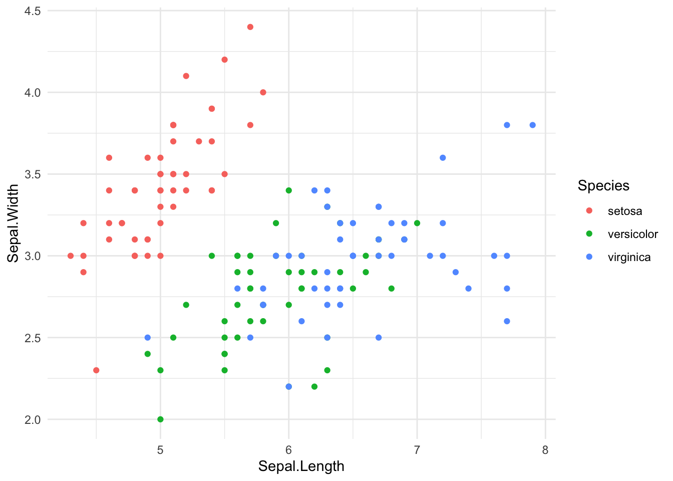
ggplot(iris) +aes(x = Sepal.Length, y = Sepal.Width, color = Species) +geom_point() +theme_minimal()
Run ?sapply in your R console to see the documentation for this function.↩︎