3 RStudio Essentials
3.1 RStudio IDE
3.1.1 Overview
3.1.2 Integrated Development Environments (IDE)
3.2 Layout
RStudio looks like a grid of four panels which you can rearrange as you like. Your source and console panels will always be two of these four. The other two panels will be one or more tabs of useful information and actions. By default, RStudio has the following pane layout:
- Top left: Source
- Bottom left: Console
- Top right tab group: Environment, History, Git, Build, and others
- Bottom right: Files, Plots, Packages, Help, Viewer, and others
You can customize how panes are grouped in tabs and where panes and pane groups appear. See Section 3.3.5 to learn how to change pane layouts. Here is my own preferred layout, which you’ll see in screenshots throughout this book:
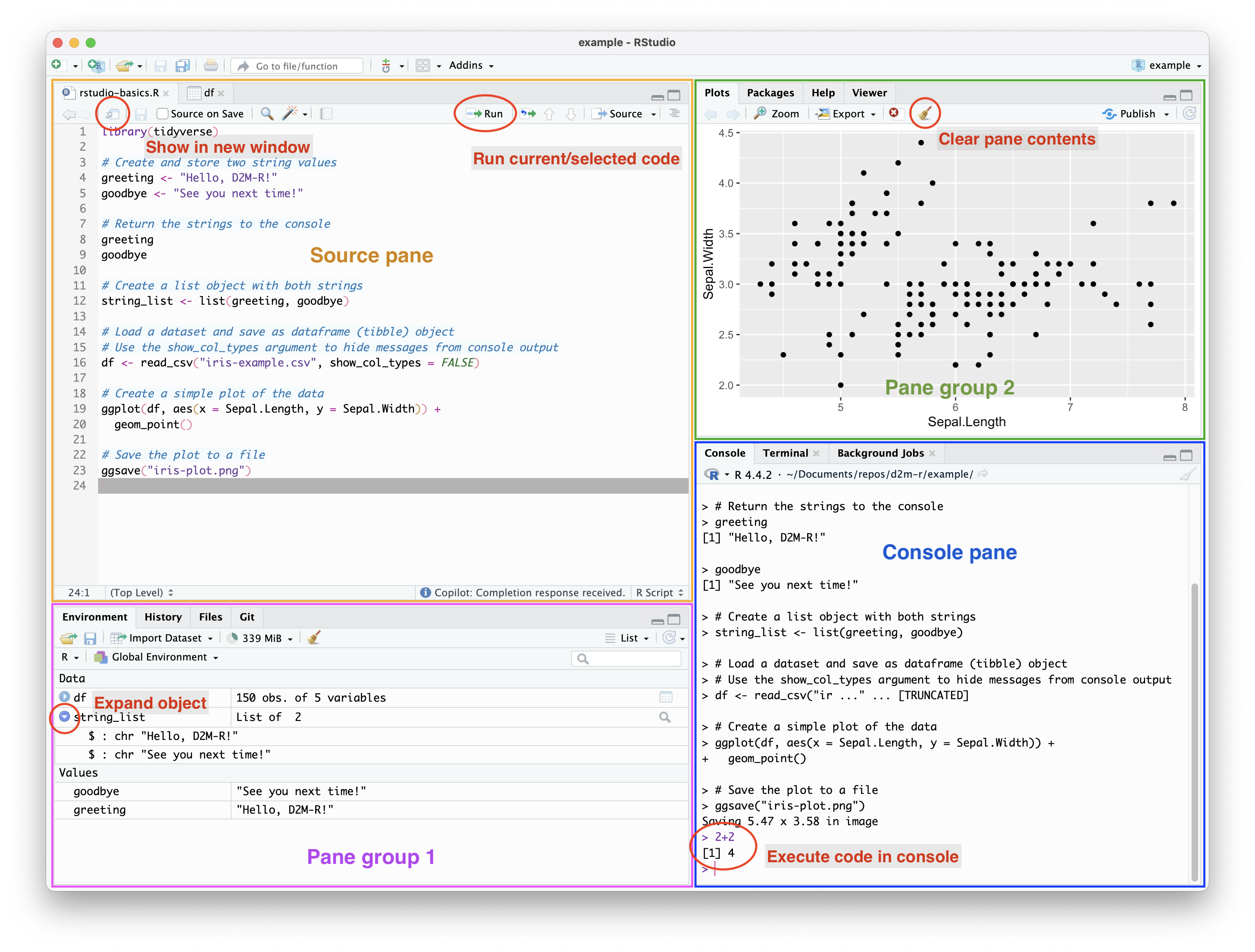
This example includes a simple R script in the source pane (top left) which has been run, producing output in the console pane (lower right) and a plot in the plots pane (top right). The objects created by the script appear in the environments pane (lower left).
3.2.1 Source pane
In both the default layout and the example layout above (Figure 3.1), the source pane is the top left quarter of the screen. Here it is outlined in orange. This is where you will view and edit the contents of text-based files, including .R scripts and markdown documents. You can also view (but not edit) contents of existing data objects in the source pane. For example, opening a stored dataframe from the environment pane or with the View() function will open it in the source pane in an easy-to-read table format.
Although you can run code directly in the console, you will most often write, edit, and run code in the source pane. The output of code run in from R scripts will appear in the console, viewer, or plot panes. The output of code in R and Quarto notebooks will appear in the document itself, below the code chunk.
There are a few important features of the source pane to be aware of:
- You can open multiple files in the source pane, and they will appear as tabs that you can switch between.
- You can pop out one or more files from the source pane using the “show in new window” button. This is useful if you want to view multiple files side by side. I often pop out simple text/markdown files to have as a reference, but leave any files that output to the console pane in the source pane.
- You can run code directly from the source pane by selecting the code you want to run and pressing
Cmd + Enter1, or by clicking the “Run” button in the toolbar above the source pane. - If you don’t select any code, using the run shortcut or run button will execute the current line of code (wherever your cursor is).
- You can run the entire file by pressing
Cmd + Shift + Enter.
3.2.2 Console pane
In Figure 3.1, the console pane is the bottom right quarter of the screen, outlined in blue. In the default layout, it is the bottom left quarter of the screen, below the source pane. The console pane has three tabs: console, terminal, and background jobs. Note that all of these tabs together make up the console pane. The “R console” refers to the console tab within the console pane.
3.2.2.1 Console tab
When you run a line of code in your source script file, it will execute in the console tab. If you select a section of code and run it, you’ll see that code appear in the console, then the output will appear immediately below it.
If something goes wrong, or if there’s just something R thinks you should know about the code you’re running, you’ll see an error, warning, or message as well.
You can also run code directly in the console tab without using a source script. Just type in some R code into the console and press return to run it. You’ll see more or less the same behavior as when you run code from a source script: the code appears (or rather, it appeared as you typed it) and the output appears below.
Run the following lines of code in the console to try it out. For multiline blocks, try both running each line one at a time and copying and pasting the entire block at once. Pay attention to both where the output appears and when it appears (or really, when it does not appear). The comments (# Which look like this) are there for you-the-human, not R. When R executes the code, it ignores everything on the line after #. You can include the comments or not, up to you.
# Some simple math
2 + 2
# Assign a numeric value to a variable and then use it
x <- 5
x * 2# Create a vector and calculate the mean
# Both directly and using a variable
my_numbers <- c(1, 2, 3, 4, 5)
mean(c(1, 2, 3, 4, 5))
mean(my_numbers)# Print a message with a string
print("Hello!")# Assign a string to a variable and print it
hello <- "Hello!"
print(hello)Running code directly in the R console is useful for quick calculations, testing small snippets of code, and some simple data exploration. Critically, the console does not save your code when your R session ends2, so you should not use it to run any code that you anticipate needing to run more than once or that may require editing.
A table for quick reference of when to use a source script and when to use the console:
| Use Case | Source Script | R Console |
|---|---|---|
| Quick calculations | No | Yes |
| Playing around with new functions | No | Yes |
| Line-by-line debugging | Yes | Yes |
| Testing small code snippets | Yes | Yes |
| Exploratory visualization | Yes | Yes |
| Exploratory data summary | Yes | Yes |
| Creating objects and functions | Yes | No |
| Data wrangling & preparation | Yes | No |
| Creating publication-ready plots | Yes | No |
| Running reproducible analyses | Yes | No |
There’s really no situation where you absolutely should not run code from a script. There are simply contexts where you may prefer not to. When in doubt, just run your code from a script in the source pane.
One more thing to notice now is the broom icon in all three tabs. You’ll actually see this icon in most panes (other than the source pane). In Figure 3.1, one example of the broom icon is circled in the plots pane in the top right. The broom icon does basically the same thing in all panes: it clears the output of the current tab. Very handy for long coding sessions, where console output gets cluttered with messages, old broken code, and other distracting things you don’t need to see anymore.
Learn more:
3.2.2.2 Terminal tab
The terminal tab is a command line interface (CLI) that allows you to run shell commands directly from RStudio.
This is where the operating system you’re using starts to matter. As mentioned, this book is written for a specific audience of students, and that audience overwhelmingly uses Mac. If you’re using Mac or Linux, the terminal tab will run commands in a bash shell by default. That’s what you’ll see in this book. If you’re using Windows, the terminal tab will run commands in the Windows Command Prompt (cmd) or PowerShell, depending on your settings. Thankfully, there are plenty of resources available online for using the terminal in Windows. To get you started, try this overview from Microsoft.
The terminal tab in RStudio functions identically to the Terminal app that runs independently. It interacts with your operating system to navigate directories, manage files, run simple text editors, and run shell commands. It does not interact with your R code.
In this course we will mainly use the terminal tab for git commands, so we cover the basics of bash scripts together with git commands in the Git & GitHub chapter (Chapter 5).
What you need to know now: The terminal tab and console tab are two different things. You can’t run R code in the terminal; you can’t run shell commands in the console. If code isn’t working at all, check that you’re in the right tab.
3.2.2.3 Background jobs tab
The background jobs tab is where you can monitor background processes that RStudio is running. Unlike the console and terminal tabs, the background jobs tab is not interactive, it is a real-time log of background processes that RStudio is running (other than code). For example, when you render a notebook with Quarto or markdown, you’ll see the processes that go into creating the document (like compiling LaTeX and markup) appear here.
What you need to know now: When you render a document, errors and warnings will appear in the background jobs tab, not the console where R code errors appear. When a job is running in the background, you can click the stop sign to force quit it. There are times when RStudio will take you to the background jobs tab automatically, so like with the terminal, just be aware of which tab you’re viewing.
3.2.3 Other commonly used panes
Aside from source and console, you can toggle panes on and off and group them together as tabs however you like. Note that even though we call them “panes” in RStudio, they are actually tabs within the larger pane layout, which is why you can customize the groups.
Before we talk details, it’s worth pointing out that many of these panes are just a GUI for R functions that you can (and usually should) run directly in the console or a source script. Can you install and load packages from the packages pane? Yes. Should you? No. You should use the install.packages() and library() functions to keep your project files and code self-contained and reproducible.
Similar things can be said about other panes or pane features: importing datasets in the environment pane, changing the working directory in the files pane, performing simple (and not so simple) git commands in the git pane, etc.
In this section, I’ll point out how to use the interactive interface for each pane, but as a student developing your R skills, you should try to learn the code equivalent for any action you take in an RStudio pane. I recommend approaching using the GUI the same way I recommend using AI. Use it as a shortcut to skip the time consuming grunt work for things you already know how to do yourself. Computers are, ultimately, pretty stupid. You need to know how this stuff actually works so you can recognize where the computer is going wrong and how to fix it.
3.2.3.1 Environment pane
In Figure 3.1, the environment pane is the bottom left quarter of the screen, outlined in purple. Here you’ll see all the objects that are currently loaded in your R session, like dataframes, variables, and functions. In order for you to reference something in your code, you have to add it to your environment first. The environment resets when your R session restarts, so you’ll need to rerun code to recreate any objects you want to use.
If you have structured objects like dataframes, lists, or model output, you can click the blue arrow to expand the object and view its component parts. You can also click the name of the object to run View(objectname). This will open the object in the source pane in either a tabular format (like for dataframes) or a nested list (like for models).
You can remove objects from your environment with the “Clear” button (the broom icon). By default, this will clear all currently loaded objects. If you just want to remove certain objects, switch from “List” to “Grid”, select the objects you want to remove, then click the broom icon.
The environment pane also has a button to import datasets. It opens a relatively user-friendly window for importing data from various file formats, like CSV, Excel, and others. This is really just assisting you in writing the R code to import the data, and you can view the code that it will run as you change import options. You can play around with this to see how different import options are represented in code, but generally when you import data you’ll want to write the code yourself to include in a source script.
3.2.3.2 History pane
The history pane is where you can see a list of all the commands you’ve run in your R session, whether from the console or from a source script. You can select a command from the history list and send it directly to the console or to the currently open source file.
You probably won’t use this pane often in your regular workflow, but it’s handy sometimes. Run something you thought was temporary in the console but now you want to keep it? Find the command and add to source. Need to rerun a quick, non-source-worthy command without scrolling up through hundreds of lines of console output? Find it in the history and run it again. Cleaned up the console two seconds before realizing you need to run that command you just ran one more time? No worries. It’s in the history.
3.2.3.3 Files pane
The files pane should be familiar to you; it’s just a directory navigator like Mac’s Finder or the Windows File Explorer. It’s not quite as pretty, but it works the same way. Navigate through folders, create new files, delete and rename, etc.
One non-obvious thing you should know is how to view and change your working directory using the “More” menu. Think of your working directory as a you-are-here marker for RStudio. When you run code that references files (like importing data, saving plots, or sourcing scripts), you need to give R a file path to that new or existing file.
You could give it a full, absolute file path (like “/Users/Natalie/Documents/repos/D2M-R/data/mydata.csv”), but that’s kind of terrible. In addition to just being a pain to type, using absolute file paths is not good practice because your code becomes less portable and harder to share with others. When you try to use my code, you probably don’t have the file in a “Natalie” folder on your computer3, so it won’t work. You’ll have to manually go in and change every file path.
Better practice is to use relative file paths. Relative to what? Relative to your working directory. If you are working in an R project, your working directory is the root of that project. If my data file is in my D2M-R project (connected to a GitHub repo), I can just use the relative file path “data/mydata.csv” to reference it. Now when you clone my repo to your own computer, you can call it anything you want and save it anywhere you want, but as long as you keep the same relative file structure, my code will still work.
As long as you’re working in an RStudio project, you won’t have to manually mess with your working directory often. If you’re not in a project, or there is just some other reason you need to change your working directory, you can do so in the files pane by navigating to the desired folder and clicking the “More” button, then “Set as Working Directory”.
All of this is really just a GUI way of doing the same thing as the setwd() function in R or the cd command in the terminal.
3.2.3.4 VCS (Git) pane
If you have a version control system (VCS) like git enabled for an RStudio project, you can enable a VCS pane. I’ll call it the Git pane, since that’s the most common VCS used with RStudio and what we’ll use in this course.
The git pane allows you to perform most basic git operations directly from RStudio. We’ll go over the git pane in detail in the Git & GitHub chapter (Chapter 5), but there are some basics you can get familiar with now.
What you actually see displayed in the git pane is a list of files that have been changed since the last commit. This includes edits to the text, additions, deletions, and renaming. You can select modified files (or directories) to stage them, so that their changes are included in your next commit. When you’re happy with what you’ve staged, click the “commit” button. A window will pop up where you get more information about what you’re staging and let you complete the commit. In that window you can add and remove items from the staging area, view the version comparison diff, add a commit message, commit, and pull/push to a remote repository. You can also switch from “Changes” to “History” to see a list of all the commits made to the project so far.
I list all those things out because – as you may have noticed – they are the same functions as the buttons at the top of the git pane. The buttons are a little deceptive, because they all open the same window. The push and pull buttons can perform those actions on their own, but everything else will just open up that same git interface window.
Another thing to mention at this point is that the git pane is great, but somewhat limited. We can do everything in a standard workflow via the git pane, but when things inevitably go wrong, you may not be able to resolve your problem in the RStudio git pane or window. In addition to being comfortable working in the git pane, you’ll need to know some basic git commands to resolve issues in the terminal.
3.2.3.5 Packages pane
The packages pane is where you can manage the R packages installed on your computer. I do not recommend installing or loading packages directly from the pane, but you can. Click install to open a window where you can search for packages, select them, and install them. Click the checkbox by a package to load it into your R session. But also, well…don’t do that. Just use the install.packages() and library() functions in your source scripts.
Some of the other things you can do in this pane are very useful, though. Aside from just having a quick reference to what packages you have installed and loaded, you can keep track of which packages are up to date and quickly update many at a time as needed.
Click the name of the package to open the package documentation in the help pane. Click the globe4 icon to open the package’s website in your browser, if one is available.
3.2.3.6 Help pane
Speaking of documentation, the help pane is where you’ll find documentation for R functions, packages, and other resources. Click the home icon to find a collection of resources about R and RStudio. You can search for documentation for a specific function or package by typing its name into the search bar. You’ll only see autocomplete selections for packages and functions that you have loaded, but you can type in anything you want and it will search for the term in CRAN documentation. (We’ll talk more about CRAN in ?sec-solving-problems).
You can also access help documentation by typing ?function_name or help(function_name) in the console. It will bring up the documentation for that function in the help pane, the same as if you searched for it.
3.2.3.7 Viewer pane
The viewer pane is where you can rendered and interactive content like HTML files, Shiny apps, and dynamic visualizations. When you create something with Quarto in this class, it will typically open in the viewer pane by default. You can pop out the contents of the viewer pane to your default browser by clicking the “Open in Browser” button next to the broom/clear icon.
3.2.3.8 Plots pane
The plots pane is (unsurprisingly) where you’ll see plots and static visualizations created in R. When you run a plotting function from an R script or the console, the output will appear here. The plots pane offers some basic functionality for interacting with plots, like zooming in, exporting the plot to a file, and clearing the plot output. As with most everything else described in this section, you can also do all of this from the console with functions like ggsave() and plot().
Note that plots generated in R and Quarto notebooks will appear in the document itself, just below the code chunk that generates them. You can change this default behavior by selecting “Chunk Output in Console” from the gear icon in the source pane of the notebook document. As you might expect based on the wording of the option, this won’t just change where plots are displayed. It will display output of code executed in code chunks to the console instead of the document itself. This kind of defeats the purpose of working in a notebook in many ways, so I recommend sticking with the default unless you have a strong personal desire to change it.
3.2.4 More panes
These panes won’t be used as much in this class, but you can toggle them on and off as needed:
- Connections pane: This pane is used to manage connections to databases and other data sources. You can connect to databases like SQLite, MySQL, and PostgreSQL, as well as other data sources like Google Sheets and AWS S3.
- Personally, in my own interactions with SQL database in R I prefer to stick with writing out the code with something like the DBI package. I honestly just find the connections interface confusing.
- Build pane: This pane is mostly just a button. When you’re working in certain kinds of projects, like this very Quarto book, you can click the “Build” button to render the project. This will run the build processes necessary to render to the desired output, and you’ll see the ongoing log of those processes in the background jobs pane. The rendered project will open in the viewer pane, browser, or another app like Word or Acrobat, depending on the kind of project.
- The render/build button in the build pane has nearly the same functionality as the render/build button in the toolbar above the source pane. The main difference is that rendering from the source will render the currently open file, while rendering from the build pane will render the entire project.
- The build pane won’t appear if you aren’t working in a project that has a build process defined. I find that sometimes the build pane just doesn’t appear in projects even when it is supposed to. You can always build Quarto projects directly from the terminal with
quarto render, so don’t work too hard at getting the build pane to appear if it doesn’t.
- Presentations pane: This pane is used to view Quarto presentations, like the ones I use in class. It will only appear if you have a Quarto project open that contains a presentation file (like a .qmd file with the
format: revealjsoption in the YAML header). - Tutorial pane: RStudio has a built-in tutorial system called
learnr. We won’t use it, but you can play around with it if you like. There’s not much else to do with the tutorial pane.
3.3 General Settings & Expected Behavior
RStudio is extremely customizable with options and keyboard shortcuts, and you can set it up to work the way you like. You can ignore most of the settings for now, but there are a few that you should be aware of from the start. You don’t need to customize everything now, but you should know where to find the settings, what they do, and how to change them later.
Many of my descriptions will be accompanied by a take-home “What you need to know” (WYNTK) line. Take that for what it is; you need to know it.
3.3.1 Global vs. Project Options
RStudio has both global options (which apply to all projects) and project-specific options (which apply only to the current project). You can access these settings through the “Tools” menu. When it comes to initial setup of RStudio, you’ll want to focus on the global settings first. You can then adjust project settings as needed.
This section will walk through the most important global options to get started in D2M-R. The screenshots are directly from my own RStudio, so you can see which options I use (though you don’t need to use the same setup!).
3.3.2 General
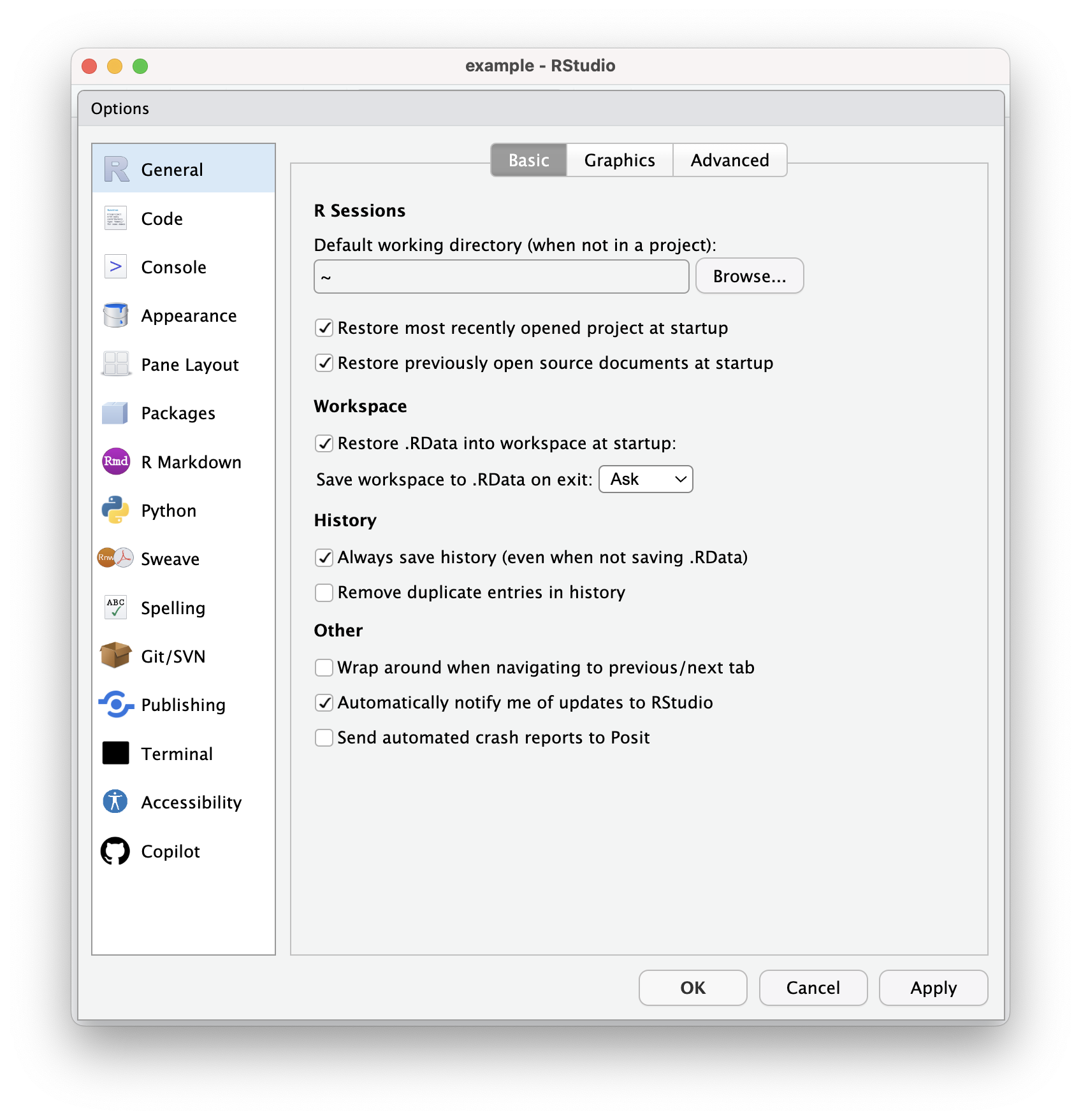
The general options do, well, general stuff. You can just worry about the “Basic” tab to get started:
- Working directory: Select a sensible folder to set as your default working directory. By default this will be your home directory (“~” is a stand-in for “/Users/YourName/”). In this class you’ll organize work in R projects, which have their own working directory. I recommend containing those projects (i.e., repositories) in one directory, and setting that as your working directory, e.g., “~/Documents/repos/”.
- WYNTK: Choose something and remember what you chose.
- Restore: Do you want RStudio to start fresh with no project and/or no documents open each time you open it, or do you want it to pick up where you left off?
- Other: Check the box to get notifications of RStudio updates. You want them.
3.3.3 Code

- Tabs or spaces: Whether to use tabs or spaces in programming is an absurd and timeless debate. R is a whitespace-insensitive programming language, meaning any kind of blank characters (both spaces and tabs) are helpful for readability but don’t matter for running the code. Use spaces, use tabs, use nothing (well, use something — human people need to read your code!). It may just be a matter of form rather than function, but you’ll likely develop a preference here. Personally I check the box and use a tab width of 4.
- WYNTK: Even though R is whitespace-insensitive, markdown is not. Since you’ll be working in Quarto notebooks in this course, you need to pick something and be consistent. If you end up with a mix of 2-space tabs and 4-space tabs (or anything else) markdown elements like lists will get wacky when you render.
- Matching parens/quotes: R uses parentheses
(), single quotes', and double quotes"to section off elements in code and markdown. It’s critical for execution that each opening paren or quote is matched with a closing paren or quote. It’s so critical, that RStudio will just go ahead and add that closer when you add an opener. This is generally preferred behavior and I recommend using it even if it takes a bit to get used to, but you can disable it if you find it distracting. - Use native pipe operator: By default, the
Shift+Ctrl/Cmd+Mkeybind inserts a magrittr (tidyverse) pipe:%>%. You’ll become very familiar with the pipe once we get to tidyverse programming. The newest versions of tidyverse packages support (and recommend) use of the native (base R) pipe operator:|>. As of 2021’s R 4.1, the two pipes are interchangeable in tidyverse functions, but|>is preferred since it will work with non-tidyverse code. Importantly, the%>%pipe still works and isn’t going anywhere, so you can use it if you want. Most of my example code (and real code for my own research) uses%>%as I gradually switch over.- WYNTK: Both
|>and%>%are pipe operators. With the tidyverse libraries loaded, you can use either. When you see them, know that they don’t have different meanings.
- WYNTK: Both
- Other editor preferences: Auto-intent to match multiple indentation on multiple lines, soft-wrap to see all your text, make the next line a comment if you hit enter while writing a whole-line comment…you can figure this stuff out.
- Keybindings: We’ll talk about keybindings a little later, but notice that this is where you can select a default set of keybinds and modify specifics.
- Ctrl+Enter: This keybind (and
Cmd-Enteron a Mac) is particularly useful. If you’re working in a source script, it will execute the “current” code where your cursor is. You can change what counts as “current.” I recommend “Multi-line R statement,” which means that R figures out the top function container your cursor is within and runs it from start to finish.- WYNTK: Get used to this keybind! Whatever setting you choose, you should use this shortcut to execute code from your source. You should not be continually selecting text with your mouse and clicking the run button.
- Snippets: More on snippets later, but this is where you turn them on and off.
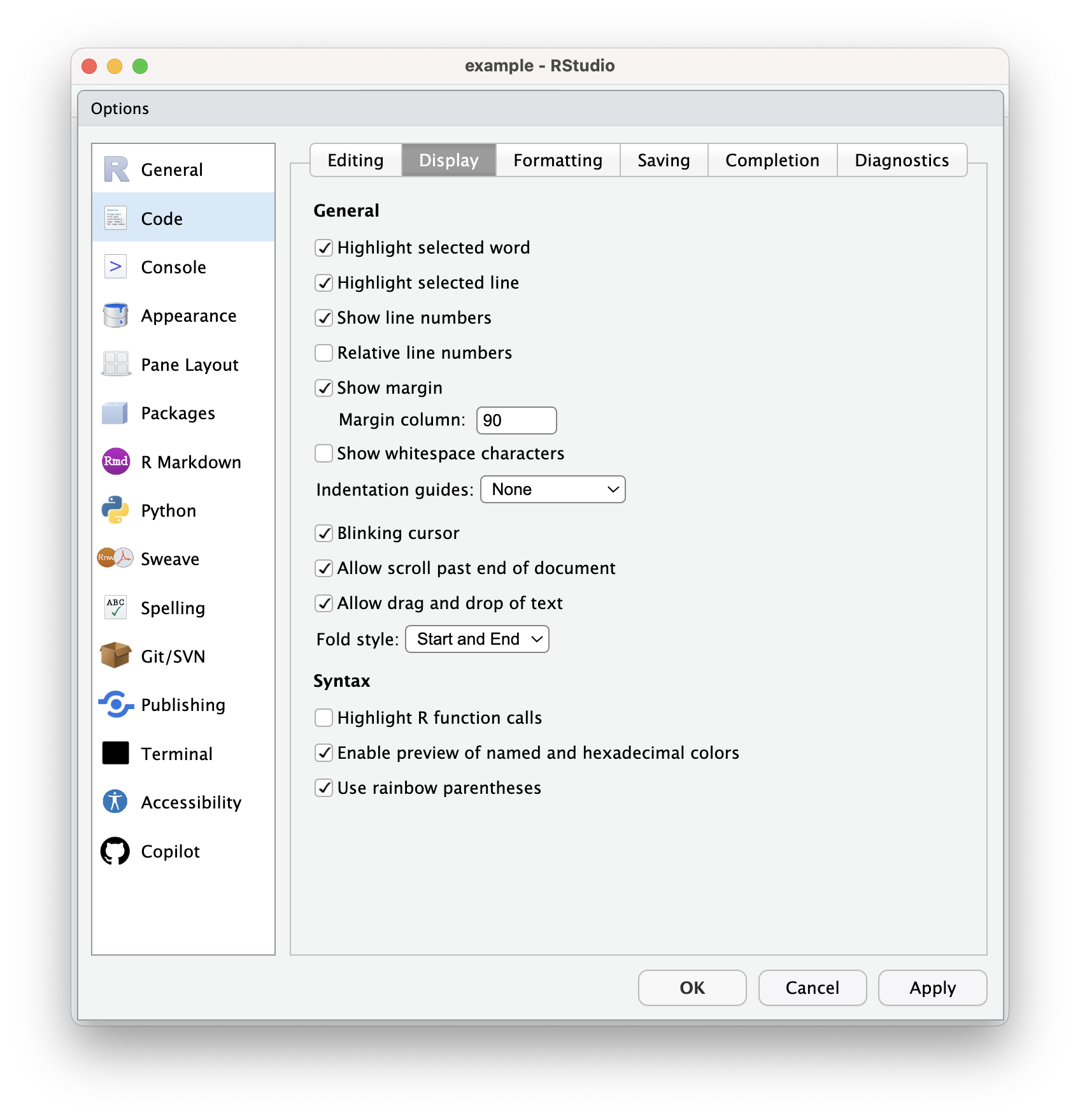
This is visual stuff that makes it easier for your individual human brain to work in text files in RStudio. You can play around and figure out what these settings do and what you prefer. Only a couple need-to-know things here:
- Show line numbers: Enable this. This is critical for your own sanity and for being able to communicate anything about your code.
- Show margin: Recall that R is whitespace insensitive, so that you can hit return to start a new line anywhere you could/should insert a space. Markdown is whitespace sensitive, but it is insensitive to single line breaks in regular blocks of text (i.e., not always in all other markdown elements like headings and lists). You can have RStudio display a vertical line to give you a visual cue of a maximum character length for each line. This is completely arbitrary and for readability only, but very handy. It’s especially useful for any documents that will display literal code blocks or other elements that will run beyond normal page margins.
- Enable color previews: When you are writing colors into code (think plots), RStudio can highlight the text naming the color in the color itself. Like, “lightblue” or “#add8e6”. Very handy, especially if you want to play around with subtle(ish) hex variations.
- Use rainbow parentheses: This will make matching sets of parentheses appear in different colors as they are embedded within each other like: ( ( ( ) ) ). Most themes will do this for you automatically.
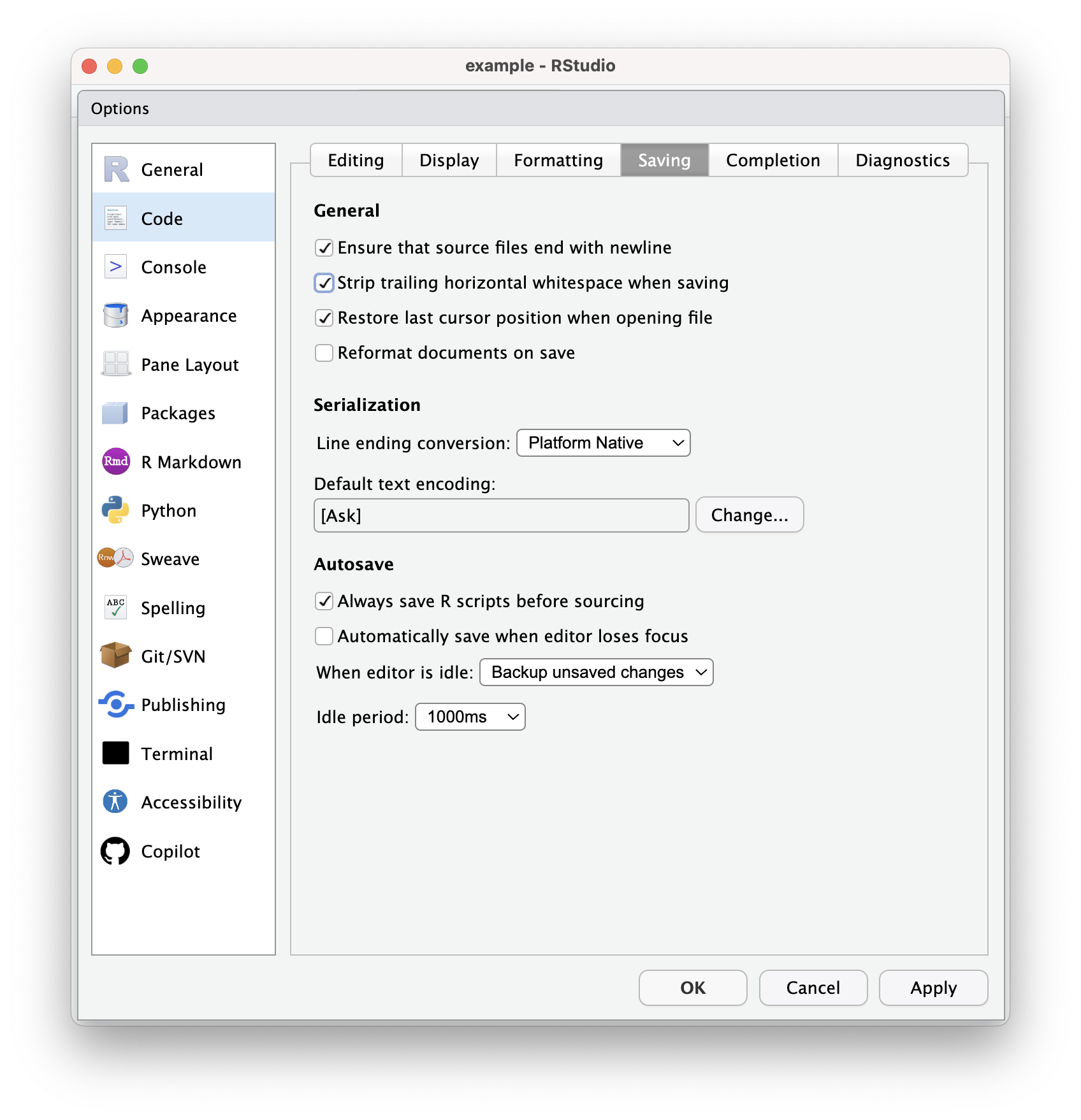 Mostly self-explanatory. WYNTK: There are autosave settings that you can use if you want. If you rely on autosave, don’t forget that you still need to make frequent commits!
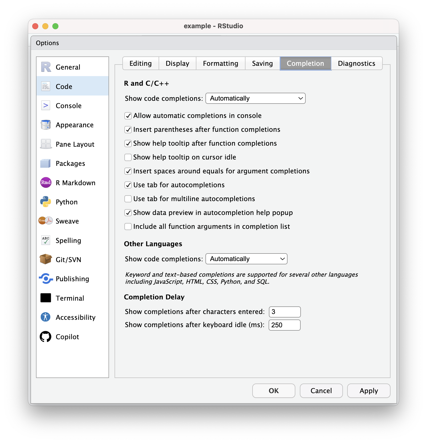
RStudio will offer autocompletion options in R scripts. This is different from Copilot suggestions, which is an AI’s best guess at writing the next bits of your code. This autocomplete is looking at the letters your typing and searching a dictionary of all available functions from base R and loaded packages. You can scroll through them with arrow keys and press tab to complete them.
3.3.4 Appearance
3.3.5 Pane Layout
3.3.6 Package Management
3.3.7 R Markdown
3.3.8 Git/SVN
3.3.9 Copilot
3.4 Additional Customization
3.4.1 Keyboard shortcuts
3.4.2 Accessibility
RStudio offers a modest set of accessibility features like screen reading and announcements that you can adjust for your own needs. At this point the accessibility options aren’t exactly robust, but they are improving with new releases, so keep an eye on this set of options if there are features you need that are not yet available. Check out Posit’s Accessibility Guide for more up-to-date info on this front.
Remember that you can use keyboard shortcuts and appearance options to improve accessibility even if there isn’t something directly available in the accessibility settings. RStudio also (generally) plays nicely with system accessibility features set from your Mac or PC settings.
3.4.3 Snippets
3.5 File types
RStudio works with many file types (including any text-based files), but there are a few that you’ll use more than others. We’ll go over each in detail as they come up in the course, but here’s a quick overview of the most common file types you’ll encounter in RStudio:
- .R: The R script file type. This is where you’ll write and save most of your R code, at least until you become a Quarto notebook devotee.
- .md: The markdown file type. Markdown is a family of markup languages, allowing you create formatted documents using plain text syntax. Common things you’ll see styled in a markdown file are heading levels (using
#,##,###, etc.), text styling (like*italics*and**bold**), and links ([link text](https://example.com)). - .Rmd: The classic R notebook that combines code and markdown. Rmd = R + md. R notebooks include a YAML header to set document options (more on that later), plain text that will use pandoc to render markdown syntax into formatted text, and code chunks that will run R code and display the output in the rendered document. You can also include code directly in the markdown text to dynamically reference R objects. This will be a major part of the second half of this course!
- .qmd: The Quarto notebook file type, which function very, very similarly to R notebooks. Quarto is branded as “R Markdown 2.0” by Posit (the makers of RStudio), and it’s replacing R Markdown moving forward. If you are already a dedicated R Markdown user and don’t want to change your ways, thankfully Quarto notebooks have backwards compatibility with everything that’s always existed in R Markdown. Quarto notebooks just offer new features and enhancements.
- There are some minor differences in general formatting norms and best practices, but in 99.9% of cases you should be able to take an .Rmd file, save it as a .qmd, and have no loss in functionality.
- In D2M-R, we use Quarto notebooks instead of classic R notebooks. As of this point I’ll refer to Quarto (instead of “Quarto and R Markdown”) and Quarto notebooks or .qmds (instead of “Quarto and R Notebooks” and “.qmd and .Rmd” files) for simplicity. Know that if you are sticking with .Rmds, most things are interchangeable, but some new features and stylings will only work in .qmd files.
- .Rproj: The R project file type is a special file associated with each R project you create that contains meta-information about that project, like its working directory, project options, and other settings. The .Rproj file will be created automatically when you create a new project. If you try to open the .Rproj file, it will open the full project in RStudio, but you can also open it in a text editor to view and edit the contents.
All of the above are the extensions to file types, but there are also a handful of metadata files and folders you should be aware of which will (or at least can) generate automatically, though you can mostly ignore them. You should actually literally ingore them by adding them to your project repo’s .gitignore file.
The “.” at the beginning of these files and folders indicates that they are hidden files; they aren’t the extensions that come at the end of file names.
- .Rproj.user: A directory of temporary files that maintains the state of your RStudio project, like what files you have open when you exit your session.
- .Rhistory: This file stores the history of commands run in the R console for the current project. It is automatically created and updated as you run commands and used to define which previous commands you can access with up and down arrows in the terminal.
- .RData: This optional file can store objects in your environment between R sessions. You have to enable it in your options. If you’re working on a project collaboratively (or, say, a project that someone may need to clone from GitHub to grade), it’s not a great idea to use this, since it won’t be consistent.
- .Rprofile: This file can contain R code that runs automatically when you start an R session in the project. Again, not great for collaborative projects.
3.6 Guided Exercise
Basic navigation in RStudio. Create a file from the files pane and in the terminal. Check and change your working directory with the files pane, the console, and the terminal. Install and load libraries using the console and the packages pane. Do some math in the console. Look up function documentation and read it in the Help pane. Write simple code in the source pane and run it directly. Run a function from the history pane. Create a Quarto document, add some markdown text, add a code chunk. Run a code chunk in the Quarto document. Render the Quarto document.
As a reminder, this book presumes use of Mac OS. Documentation for shortcuts and interface actions for Windows and Linux is plentiful elsewhere, including the Posit website↩︎
Your console input is temporarily saved in the history tab. More on that in Section 3.2.3.2.↩︎
Unless your name is also Natalie, I suppose.↩︎
Is that supposed what it’s supposed to be?↩︎